ML Interview Q Series: What is the difference between Normalization and Scaling?

📚 Browse the full ML Interview series here.

Comprehensive Explanation

Normalization generally refers to transforming your data so that each observation or feature is restricted to a specific range or has a certain property (like a unit norm). Scaling (often called standardization in many contexts) usually involves reshaping the distribution of your feature values so that they align around a common center (for example, mean 0) or standard deviation (for example, 1). Both techniques aim to ensure that different features contribute appropriately to machine learning model training, especially for distance-based or gradient-based algorithms.

Normalization Concepts

Normalization typically seeks to ensure that the values of a feature lie within a particular range, such as [0, 1] or [-1, 1]. One popular method to achieve this is Min-Max Normalization. A frequent confusion arises because Min-Max Normalization is also referred to as Min-Max Scaling in some literature. However, in practice, when many people say "Normalization," they usually mean a transformation that restricts the data into a confined interval like [0, 1].

Below is the common Min-Max Normalization formula:

Here, X represents the original feature value, min(X) is the minimum observed value for that feature in the dataset, and max(X) is the maximum observed value for that feature in the dataset. The result is X_normalized which lies between 0 and 1.

Another type of normalization is L1 or L2 normalization, often applied on rows (observations) in tasks such as text classification with TF-IDF vectors. In that scenario, each sample is normalized so that the sum or the Euclidean norm of its values is 1, preventing any row from dominating due to magnitude alone.

Scaling Concepts

Scaling often refers to methods that adjust the distribution of each feature so that its mean and standard deviation match certain desired values. The most typical approach is Standardization, where you transform each feature so that it has mean 0 and standard deviation 1 across samples. The usual formula for this method is:

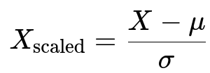
Where X is the original feature value, μ is the mean of that feature in the training dataset, and σ is the standard deviation of that feature in the training dataset. This transformation ensures the bulk of the feature values center around zero and have a standard deviation of one, which is especially helpful for algorithms that rely on gradient descent or that assume data is normally distributed.

Sometimes, in the literature or in practice, the word "scaling" is used generically to mean a variety of transformations, including min-max normalization. In that sense, "scaling" might be any transform that compresses or stretches the feature range or distribution. Nonetheless, a common convention in technical discussions is:

• Normalization = bounding or constraining values to a specific range (often [0, 1] or [-1, 1]) • Scaling = adjusting to a specified center and spread (for example mean 0, standard deviation 1)

Why the Distinction Matters

• Normalization is often chosen when the exact bounding of features is important. For example, neural networks with sigmoid activations or certain image processing tasks can benefit from having all input data in [0, 1]. • Standardization (a common form of scaling) is often chosen when you want to ensure all features have the same variance scale. This approach is helpful for methods like Principal Component Analysis, linear/logistic regression, and many distance-based algorithms such as K-NN.

In practice, these transformations can yield different results for machine learning models, especially if outliers are present:

• Min-Max Normalization can be heavily affected by outliers, since the entire range is dictated by min and max. • Standardization is somewhat more robust, but it can still be influenced by large outliers because the standard deviation might become inflated. • Robust scaling techniques (like subtracting the median and dividing by the interquartile range) are often used to mitigate outlier impact.

Practical Python Example

Below is a quick illustration of how to perform Min-Max Normalization and Standard Scaling using scikit-learn:

import numpy as np
from sklearn.preprocessing import MinMaxScaler, StandardScaler

# Example data
X = np.array([[1, 50],
              [2, 40],
              [3, 60],
              [4, 55],
              [5, 45]]).astype(float)

# Min-Max Normalization
min_max_scaler = MinMaxScaler(feature_range=(0, 1))
X_normalized = min_max_scaler.fit_transform(X)
print("Min-Max Normalized:\n", X_normalized)

# Standard Scaling
standard_scaler = StandardScaler()
X_scaled = standard_scaler.fit_transform(X)
print("Standard Scaled:\n", X_scaled)

In the snippet above, the MinMaxScaler forces data into [0, 1], while the StandardScaler centers the data at mean 0 with standard deviation 1.

How They Are Used in Practice

• If you suspect that distances between data points will be a crucial factor (like in K-NN or clustering), bounding the features to the same range (e.g., [0, 1]) often helps. • If you have features on widely different scales, standardization often helps certain models (like linear regression, neural networks, or PCA) converge more reliably. • If the presence of outliers is strong, you might consider robust scaling methods.

Potential Follow-up Questions

How do you decide when to use Normalization or Standard Scaling in practice?

You should consider the nature of your data and the algorithm you’re using. If your algorithm is sensitive to the range of the input (like K-NN), Normalization to [0, 1] might be beneficial. If your goal is to handle large numeric ranges or features that might have heavy tails, Standard Scaling can be more stable, because it focuses on the mean and standard deviation rather than just the min and max values.

What if the data contains significant outliers?

Min-Max Normalization might not be appropriate because min and max values can be heavily influenced by outliers, compressing the distribution of most data points into a narrow interval. Standard Scaling can still be influenced by outliers through its effect on the standard deviation. In such cases, robust scaling methods (using medians and interquartile ranges) can be more resilient.

Do Normalization or Scaling always improve performance?

Not necessarily. While many machine learning algorithms benefit greatly from features being on the same scale (especially those reliant on distance metrics or gradient-based optimization), some models like decision trees and random forests are not strongly affected by feature scaling, because they split on feature thresholds. It’s always best to experiment and validate with your specific dataset and model to determine whether normalization or scaling yields performance benefits.

Does normalization mean the same thing in every context?

No. Although “normalization” often refers to mapping values to a constrained range, in some contexts (such as data preprocessing in text analytics), “normalization” might refer to dividing by norm(L1 or L2) so that each vector has length 1. In other domains, you might see “normalizing by the total sum” or “normalizing by maximum frequency.” Always clarify which form of normalization is intended when discussing it with a team or reading documentation.

Below are additional follow-up questions

How do you handle feature columns that are recorded in different units or scales?

When real-world data comes from diverse sources, it is common to see features recorded in widely different units. For instance, one feature might be the number of clicks on a website (typically in tens or hundreds), while another might be the user’s average session duration in seconds (which can be in thousands), and a third might be the user’s device screen size in inches. If these units are not converted or scaled properly, a learning algorithm could inadvertently assign disproportionate influence to features with larger absolute values.

A subtle pitfall arises when some features have extremely large or small numerical ranges compared to others. Even after scaling, occasional spikes in the “large-scale” features may overshadow normal fluctuations in the “small-scale” features. Carefully examining your data to ensure that all features align in a way consistent with your model’s assumptions is crucial. Sometimes domain knowledge suggests that you should convert one feature from seconds to hours (or vice versa) before deciding on the best normalization or scaling approach. Failing to do so might cause certain models, like K-NN or SVM, to be biased toward certain features purely because of magnitude differences, rather than because those features are more predictive.

How should we deal with new data that has values outside the range of our original training set if we used min-max normalization?

In a training setting, min-max normalization depends on the min and max values of each feature in the training set. After fitting, new data might contain observations that exceed these original minima or maxima. If you simply apply the same min-max formula, any value that is larger than the original max will produce a result greater than 1, and any value smaller than the original min will produce a result below 0. This can cause unexpected behavior in models that assume normalized inputs strictly lie in [0, 1].

One common strategy is to clip any values that exceed the original bounds to 0 or 1. Another approach is to update the min and max values in an online fashion if your use case allows it. However, updating the min and max for the entire feature distribution dynamically can cause inconsistencies over time, especially if you’re retraining models in a streaming environment. Some practitioners prefer robust scaling methods or standard scaling when they anticipate new data can lie outside the previous training range.

Do we recalculate scaling parameters (mean and std or min and max) for each batch or do we fix them from the training set?

In a typical training and production pipeline, you fit your scaler (whether min-max normalization or standard scaling) on the training set alone. The resulting parameters—mean, standard deviation, min, and max—are then fixed for all future data. Recomputing these statistics on each batch of test data risks data leakage (where knowledge of the test distribution contaminates training) and also makes the model’s interpretation inconsistent across different batches.

An edge case occurs when you need to adapt to shifts in incoming data distribution (like in non-stationary or streaming scenarios). You might choose to continuously update your scaling parameters to keep pace with the evolving data. However, this approach can introduce stability issues if your data drifts slowly over time and you keep changing the parameters. A compromise is to employ a rolling or exponentially weighted average to track the distribution while keeping the changes small and controlled.

When would you consider using a log transformation or power transforms instead of standard scaling or min-max normalization?

Sometimes, features show heavy skew or follow a long-tailed distribution. Simply applying min-max normalization or standard scaling might not address the underlying skew. A log transform, for instance, can compress large outliers if the data is strictly positive. Power transforms (like the Box-Cox or Yeo-Johnson transformations) similarly aim to make the distribution more Gaussian-like.

A real-world example might be financial data on sales or revenues, where 90% of data points cluster below a certain threshold, but 10% can be extremely high. If you directly apply min-max normalization, that handful of outlier points sets a very large max, causing most data points to collapse near 0. A log transform can reduce this extreme imbalance. Nonetheless, a key pitfall is that you need non-negative data for log transforms (or else you must shift the data if it contains zeros), and interpreting model outputs can be trickier if you forget you took the logarithm.

How do you manage normalization or scaling for online learning or streaming data?

In online learning, data arrives sequentially, and you might need to update your model incrementally. For instance, in stochastic gradient descent, you feed new observations one (or a few) at a time. If you rely on standard scaling, you cannot simply store all your data to recalculate the mean and standard deviation each time. Instead, you maintain running estimates of these statistics. This process can be done using incremental formulas for mean and variance.

A challenge emerges if your data undergoes abrupt distributional shifts (for example, new users behave quite differently from older ones). A naive approach that lumps all data together might produce a scaling factor that is no longer optimal. You might incorporate forgetting factors or time windows to allow your scaling parameters to adapt slowly. However, if you adapt too aggressively, your model might overreact to short-term fluctuations. Balancing these considerations is key in practical streaming or online scenarios.

Do tree-based ensemble methods require normalization or scaling?

Methods like random forests and gradient-boosted decision trees split on feature thresholds without depending on Euclidean distance or gradient magnitudes in the same way that linear methods do. As a result, decision trees generally do not require normalization or scaling to achieve good performance. You can train a random forest on raw data with widely varying feature scales and still get valid splits.

However, there are some caveats. If you are using decision trees along with other algorithms (for instance, in a voting or stacking ensemble), then having consistent preprocessing across all models might simplify your pipeline. Moreover, if the range of feature values is extremely large, certain software implementations might still face numerical instability or computational inefficiency, making some form of scaling beneficial. But strictly from an accuracy standpoint, classic tree-based methods are generally robust to the absolute scale of the features.

What is the effect of normalizing the entire dataset at once versus normalizing each feature individually?

In most standard practices, you normalize or scale each feature (column) independently of others. For min-max normalization or standard scaling, you compute parameters (min, max, mean, std) per feature. However, in certain specialized tasks (like image processing), people sometimes normalize entire images by a single mean and standard deviation across all pixels (especially if the problem is sensitive to global brightness or contrast).

Applying a single normalization across all features merges their distributions, which might hide or distort the distinctive information each feature contains. For example, if you have two columns, one representing age (range in decades) and one representing income (range in thousands of dollars), normalizing them jointly might render the result meaningless. Each feature’s distribution has unique statistical properties, so typically you want to maintain them separately. The pitfall is that if you try a combined or global normalization, you might inadvertently throw away useful information or create features with spurious relationships.

Is it ever useful to normalize or scale the target variable in regression tasks?

Yes, there are situations where transforming the target can help your regression model. For instance, if the target variable is extremely skewed or spans multiple orders of magnitude (such as housing prices ranging from a few thousand to several million dollars), applying a log transform to the target sometimes stabilizes the training process and reduces error metrics. Doing so can also make it easier for the model to handle multiplicative relationships.

However, a pitfall occurs when interpreting the predictions. If you have trained your model on log(target), then your model’s outputs are also in log scale, which means you must exponentiate them (or use the appropriate inverse transform) to return to the original space. Forgetting this step leads to incorrect predictions or confusion. Additionally, if your data has zero or negative target values, a direct log transform is not feasible without shifting those values first, and that shift can complicate interpretability.

How do you handle missing data when performing normalization or scaling?

Most libraries (like scikit-learn) require that you either drop or impute missing values before applying normalization or scaling. A subtle real-world issue arises if you impute the missing values with the mean or median before computing scaling parameters: the imputation itself changes the overall mean (or distribution) of the data, which in turn affects the scaling. One approach is to run imputation first, then compute scaling parameters from the imputed data. Alternatively, you can compute scaling parameters using only the non-missing values, then apply the same transformations post-imputation.

The key pitfall is maintaining consistent preprocessing between training and any future data in production. If your production data has missing values, you must apply the same imputation method and the same scaling parameters derived from your training set. Deviations in approach lead to data leakage or inconsistencies that degrade model performance.

Are there specialized transformations for data subject to drift or out-of-domain inputs?

In scenarios where your data distribution may shift significantly over time or may include previously unseen patterns, specialized methods can be employed. One strategy is to use robust scalers (like the median and interquartile range) that are less sensitive to outliers or drifting extremes. Another approach is adaptive normalization, where you update your normalization parameters gradually based on incoming data. This can help the model remain stable while still adapting to a changing environment.

One subtle edge case is out-of-domain inputs: new samples that do not resemble any training data. Even robust scalers might fail if the distribution drifts too far from the original. In such cases, you might couple scaling with anomaly detection. If you detect that data is out-of-domain, you can either ignore those points or handle them differently (e.g., revise your model or re-fit your scaling parameters on an updated training set). This extra level of caution can prevent catastrophic mis-scaling that distorts your model’s predictions.