
ML Interview Q Series: What is the difference between Non-dependency and Dependency-oriented data?

📚 Browse the full ML Interview series here.
Comprehensive Explanation
Non-dependency data typically assumes that each observation in the dataset is independent of the others. This usually aligns with the i.i.d. (independent and identically distributed) assumption common in many standard machine learning algorithms such as linear regression, logistic regression, or feed-forward neural networks. On the other hand, dependency-oriented data suggests that each data point depends, to some extent, on other samples in the dataset. Time-series, sequence data, graph data, and spatial data are examples where this occurs.
When we say that data is non-dependent, we often rely on the assumption that the joint probability over all observations can be factorized as a product of individual probabilities. In simpler terms, each observation’s distribution is unaffected by any other observation’s values.
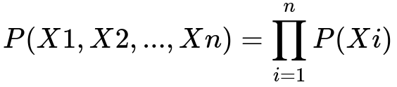
Here, each X_i is one sample, and P(Xi) is the probability associated with that sample. This assumption dramatically simplifies the modeling process because we can treat each instance in isolation without worrying about the correlations among samples. For many real-world scenarios, especially ones like tabular data where records come from independent events, this assumption is not too problematic. However, ignoring potential correlations or structures when they exist can degrade model performance or lead to incorrect conclusions about cause and effect.
Dependency-oriented data involves situations where observations are related. Examples include time-series data where the value at time t depends on the value at time t-1, or in sequence problems (like language modeling) where the next token depends on previous tokens. Graph data is another instance of dependency: node features or labels depend on the node’s neighbors. Because these dependencies violate the i.i.d. assumption, specialized models like RNNs, Transformers, Markov chains, or Graph Neural Networks are often deployed to effectively learn from such structures.
Compared to non-dependency data, modeling dependency-oriented data requires additional considerations regarding how to capture these correlations. Failing to properly account for dependencies can lead to incorrect estimates of uncertainty and model parameters. For example, in time-series forecasting, you cannot simply shuffle the data and treat each point as independent; you must maintain the chronological order or else lose valuable information about trends and seasonal patterns.
Systems dealing with dependency-oriented data are typically more complex in terms of data preprocessing and computational costs. You need to decide how much context or how many historical data points to include (e.g., time lags in time-series). In situations like social network analysis, you may need to consider local and global graph structures.
Data splitting strategies also differ. For non-dependency data, random splits suffice. For dependency-oriented data such as time-series, you must respect temporal ordering when splitting into training and validation sets to avoid data leakage from the future into the past. In graph tasks, you might consider structural splits to avoid overly optimistic validation results.
Common Real-World Examples
In many practical scenarios, you might encounter both types of data. For instance, if you are analyzing customer transactions, you can often treat each purchase as a separate observation with minimal dependency among them, especially if they occur in different markets or contexts. However, if you are studying user behavior on a digital platform over time, you must account for the fact that each user’s actions today may be influenced by their own behavior yesterday. This requires time-series or sequential approaches, or possibly user-level modeling that captures the repeated nature of interactions.
Potential Follow-up Questions
How can we detect if our data is dependent or non-dependent?
One way is to calculate correlation or mutual information between samples. In time-series data, you can plot autocorrelation functions and partial autocorrelation functions to see if past observations strongly influence the present. You can also keep an eye on domain knowledge: for example, if your data points come from repeated measurements, sensor readings over time, or connected structures like social graphs, then it is almost certain you have dependencies. When such interdependencies exist, ignoring them can lead to biased or overly simplistic models.
What modeling techniques work best for dependency-oriented data?
Sequential data typically leverages RNNs, LSTM, GRU, or Transformer-based models for tasks like time-series prediction or language modeling. Markov chain methods are also used, especially for simpler sequential patterns. For spatial or graph data, graph neural networks like GCN (Graph Convolutional Network), GAT (Graph Attention Network), and GraphSAGE can capture structural dependencies. Each of these architectures explicitly encodes the relationships or dependencies among data points—time steps, sequences of tokens, or connections in a graph—thereby helping the model learn from those relationships.
Can we convert dependency-oriented data into non-dependency data?
Sometimes you can transform dependency-oriented data into non-dependent form by carefully engineering features. For instance, in a time-series scenario, you might take lagged features from prior time steps and treat them as part of a single row, thus capturing some temporal information in a tabular form. However, this approach can lose certain long-range or more nuanced dependencies. Advanced models like RNNs, Transformers, and probabilistic graphical models are often better suited to directly model the dependency structure without flattening it into a simplistic, non-dependent format.
Are there challenges in training models on dependency-oriented data?
There can be several challenges related to computational overhead and complexity of the data representation. For time-series, you often have to watch out for stationarity assumptions and must handle seasonality carefully. In graph data, the model needs to propagate information across neighbors, which could lead to issues with computational scaling for very large graphs. Moreover, the order of training data matters, especially in time-series tasks, because you cannot randomize the sequence arbitrarily without losing the information about how dependencies progress over time.
How do we approach cross-validation differently for time-series?
Random k-fold cross-validation, commonly used for non-dependency data, would violate the chronological sequence in time-series. Instead, a more suitable approach is a time-series split (sometimes called forward chaining). You train on an initial segment of the data, then validate on the next segment, and so forth, moving forward in time without mixing future data into the training phase. This approach prevents leakage of future information and provides a more accurate assessment of how the model will perform in real temporal settings.
How do we handle non-stationarity in dependency-oriented data?
Non-stationarity occurs when the underlying statistical properties of the process generating the data change over time. You could apply methods like differencing or transformation to stabilize the mean and variance in time-series. Online learning techniques and adaptive models that update parameters regularly can also be helpful. Model selection (e.g., ARIMA, SARIMA, LSTM, or Transformer-based models) should account for whether the data generating process is stationary or not. Failure to handle non-stationarity appropriately can lead to poor forecasting performance and misguided conclusions.
Could you share a quick Python code snippet for forecasting dependency-oriented data?
Below is a minimal example of training an LSTM on a univariate time-series using PyTorch. It shows how to shape your data for a model that expects sequential input rather than non-dependent samples:
import torch
import torch.nn as nn

class SimpleLSTM(nn.Module):
    def __init__(self, input_size=1, hidden_size=32, output_size=1):
        super(SimpleLSTM, self).__init__()
        self.lstm = nn.LSTM(input_size, hidden_size, batch_first=True)
        self.fc = nn.Linear(hidden_size, output_size)

    def forward(self, x):
        out, _ = self.lstm(x)
        out = self.fc(out[:, -1, :])
        return out

# Example usage
# Suppose 'series' is a list/array of time-series values
def create_sequences(data, seq_length):
    xs = []
    ys = []
    for i in range(len(data) - seq_length):
        x_seq = data[i:i+seq_length]
        y_seq = data[i+seq_length]
        xs.append(x_seq)
        ys.append(y_seq)
    return torch.FloatTensor(xs).unsqueeze(-1), torch.FloatTensor(ys)

# Sample data
series = [float(i) for i in range(100)]
seq_length = 5
X, y = create_sequences(series, seq_length)

model = SimpleLSTM()
criterion = nn.MSELoss()
optimizer = torch.optim.Adam(model.parameters(), lr=0.001)

epochs = 10
for epoch in range(epochs):
    optimizer.zero_grad()
    outputs = model(X)
    loss = criterion(outputs, y.unsqueeze(-1))
    loss.backward()
    optimizer.step()
In this snippet, we create sequences of length seq_length from a univariate time-series. Each sequence is treated as a dependent series of observations, not independently and identically distributed samples. The LSTM is better equipped to model sequential dependencies compared to approaches that assume non-dependency data.
The key takeaway is that when data points are independent, you can apply standard machine learning approaches directly. When data points are dependent, specialized architectures and careful training/evaluation practices are critical to capture and properly model those dependencies.
Below are additional follow-up questions
How can we evaluate model performance in scenarios where dependencies exist?
When data points have inherent dependencies, traditional metrics like accuracy, RMSE (root mean squared error), or MAE (mean absolute error) may still be valid, but special care must be taken in how we gather test or validation predictions. For example, in time-series forecasting, a future data point depends on the past, so you must not shuffle the time order. Evaluating on a strictly forward-chained timeline will better reflect real-world deployment, where the model only sees the past to predict the future.
Pitfalls and Edge Cases:
Data Leakage: If you perform random train-test splitting on a time-series, the model might indirectly see future data when training, leading to overly optimistic results.
Multi-step Forecasting: In many time-series tasks, you predict multiple steps into the future. A small prediction error at one step can compound at subsequent steps. Metrics should account for this cumulative effect. For instance, you can calculate rolling predictions rather than just a single-step prediction error.
Structural Breaks: If your time-series or graph data experiences major changes in structure (e.g., new connections in a social network, abrupt regime changes in finance), evaluation might be misleading if those changes aren’t reflected or anticipated by the model.
When might we choose not to model dependencies even if they exist?
In certain practical scenarios, the cost or complexity of modeling dependencies might be too high relative to the improvement gained. For instance, if your dataset is large, but the dependency is weak, capturing it might not yield a substantial performance boost, whereas simpler models with fewer parameters might suffice. Similarly, in operational constraints (e.g., real-time prediction on limited hardware), a heavy sequence model might be impractical, so a simpler method ignoring mild dependencies could be the pragmatic choice.
Pitfalls and Edge Cases:
Underestimating the Value of Dependencies: Sometimes, a slight correlation can become significant in rare or edge cases. By ignoring dependencies, you might miss out on important cues that could drastically affect performance in critical applications (e.g., anomaly detection in sensor networks).
Interpretability vs. Complexity: A fully interdependent model can be harder to interpret, especially if it involves advanced architectures like recurrent neural networks or Transformers. If your business requires interpretability, you might forgo sophisticated dependency modeling in favor of a simpler approach.
How do we handle missing or irregular time intervals in dependency-oriented data?
Many real-world time-series datasets have missing data points or irregular sampling intervals. This breaks the standard assumption of evenly spaced observations. You can apply techniques such as forward filling, interpolation, or more advanced imputation methods. For instance, in sensor networks, data might come in bursts, and you must decide how to align these readings to maintain the temporal sequence accurately.
Pitfalls and Edge Cases:
Bias in Imputation: Simple imputation (like forward filling) can introduce bias if the missing data mechanism isn’t random. Over long periods without measurements, forward filling can mask trends or abrupt changes.
Irregular Sampling: Some models, particularly RNNs, assume regular time steps. Irregular intervals might require timestamp-based modeling or specialized architectures that incorporate time lags explicitly (e.g., Neural ODEs or time-aware RNNs).
Data Quality vs. Modeling Complexity: If missingness is extensive or random, a more complex approach might not necessarily improve performance. You must balance the effort of elaborate interpolation with the practical reliability of simpler techniques.
How can domain knowledge guide feature engineering in dependency-oriented data?
Domain knowledge can reveal relationships that purely data-driven methods might not automatically detect. For instance, in climate modeling, physical laws or seasonal patterns can guide the creation of relevant lagged features or moving averages. Similarly, in finance, you might incorporate calendar effects or known macroeconomic indicators. Domain understanding often informs the length of the sequence context (e.g., how many previous timesteps matter) or the connectivity in graph data (e.g., which nodes truly influence one another).
Pitfalls and Edge Cases:
Overcomplicating Features: While domain knowledge can improve performance, overly engineered features might introduce noise if they aren’t genuinely relevant. Feature selection or regularization can mitigate this but may still be time-consuming.
Incorrect Domain Assumptions: Relying too heavily on domain knowledge that may not hold under current conditions (such as abrupt regime changes in financial markets) can lead to poorly performing models. Continuous revalidation of assumptions is crucial.
Stale Knowledge: In fast-evolving fields (e.g., e-commerce, social media), domain knowledge might become obsolete quickly. Your feature engineering pipeline should be flexible enough to adapt to new patterns or interactions.
What if only part of our dataset exhibits dependency while other parts seem independent?
Real-world datasets often contain both dependent and non-dependent segments. For example, you might have a time-series that behaves dependently during certain periods (like high volatility or seasonal spikes), but otherwise is relatively stable and can be treated as independent. Similarly, in a user-event dataset, events for the same user are dependent, but across different users with minimal interaction, the data might be nearly independent.
Pitfalls and Edge Cases:
Model Misalignment: A model that’s too specialized for dependency relationships might overfit the segments that are dependent but perform poorly on independent segments. Conversely, a model ignoring dependencies might fail to capture meaningful relationships in certain subsets.
Hybrid Approaches: Some practitioners adopt mixed models—one part handles the dependency segments (like an RNN for certain periods), and another handles non-dependent segments (like a standard regression model). But combining predictions from multiple models can be non-trivial and requires careful validation.
Data Drift and Switching Behaviors: The dependency structure might change over time (e.g., markets might become more or less correlated). Monitoring data drift and deciding whether to re-train or adapt the model dynamically is important to maintain performance.
What specialized regularization techniques are common for models trained on dependency-oriented data?
When dealing with sequential data or graph data, certain regularization methods go beyond standard L2 or dropout. For example, in RNN or LSTM models, recurrent dropout (dropping recurrent connections as well as the inputs or outputs) can help prevent overfitting in sequences. In graph neural networks, carefully dropping edges or node features (graph dropout) can prevent the model from over-relying on specific connections.
Pitfalls and Edge Cases:
Over-regularization: If you apply too much dropout or other constraints in a model that already has limited capacity, you risk underfitting and failing to capture meaningful dependencies.
Spatial/Temporal Smoothing: In image or spatiotemporal data, smoothing constraints (e.g., total variation regularization) can prevent the model from overfitting noise. However, excessive smoothing might remove legitimate local spikes or anomalies that are crucial for certain applications (e.g., anomaly detection).
Complex Implementation: More advanced regularization (like structured dropout in RNNs or custom sampling in GNNs) requires careful coding, debugging, and hyperparameter tuning to ensure it truly benefits the model without breaking or distorting the data patterns.
How do we prevent catastrophic forgetting when training a model incrementally on dependency-oriented data?
Catastrophic forgetting is a phenomenon where a model forgets previously learned knowledge when trained on a new sequence of data, particularly relevant in online or continual learning setups. In time-series or sequential models, you might incrementally update the model with new data as it arrives, but risk overwriting past information.
Pitfalls and Edge Cases:
Model Architecture Limitations: Simple RNNs can forget long-range dependencies. Using architectures with gating mechanisms (e.g., LSTM or GRU) or attention-based models can help mitigate this issue.
Replay Buffers: Storing a small set of past data points and mixing them into the training process (experience replay) can help the model retain old knowledge. However, storing too many examples can be computationally expensive or memory-intensive.
Domain Shift: If the underlying data distribution changes significantly over time (non-stationarity), relying on old data for replay might hurt performance by confusing the model with outdated patterns. Striking a balance between memory replay and adapting to new distributions is essential.
How do hierarchical models help in capturing multiple layers of dependencies?
Some datasets have layered dependencies. For instance, user data might exhibit dependencies within a single user’s actions over time, but there may also be cross-user dependencies in a social network. A hierarchical model (like a hierarchical Bayesian model or a multi-scale Transformer) can capture local correlations at one level and global correlations at another.
Pitfalls and Edge Cases:
Model Complexity: Hierarchical models tend to be more complex and can be prone to overfitting if there isn’t sufficient data to estimate many parameters. They may also require longer training times.
Data Partitioning: It can be tricky to decide the “levels” in your hierarchy (e.g., temporal grouping vs. user grouping, or both). Incorrectly defining the structure might obscure real dependencies or create spurious ones.
Interpreting Multi-level Dependencies: While hierarchical models can capture rich patterns, unraveling what the model has actually learned at each level can be challenging. This complicates debugging and interpretability.
What happens if dependencies are dynamic and change over time or space?
In real-world datasets, dependencies themselves might evolve. An example is consumer preferences that shift after major events, or graph connections that appear and disappear over time. Tracking changing dependencies often necessitates dynamic or adaptive models (e.g., time-varying coefficients in state-space models, dynamic graphs for social networks).
Pitfalls and Edge Cases:
Computational Overhead: Continuously updating a dynamic dependency structure (e.g., recalculating adjacency matrices for graphs as edges change) can be expensive and non-trivial to optimize at scale.
Delayed Observations: Some changes in dependencies might be noticeable only after a lag (e.g., a new social connection becomes meaningful after several interactions). Failing to capture this delay can lead to missing important transitions.
Model Drift: As dependencies change, any model trained on stale assumptions might degrade quickly. Monitoring data drift and introducing model retraining or parameter updating can help maintain relevance.