ML Interview Q Series: What modifications are required to transform a network’s Dense layer into a fully convolutional one?

📚 Browse the full ML Interview series here.

Comprehensive Explanation

A Dense (fully connected) layer multiplies the flattened input by a weight matrix and then adds a bias term. This assumes a fixed-size feature vector, which necessitates a fixed spatial input dimension in typical CNN pipelines. In contrast, a fully convolutional layer replaces the matrix multiplication with a convolution operation that can handle variable spatial dimensions. By using convolutions instead of the explicit flattening and matrix multiplication of a Dense layer, the network can operate on inputs of varying sizes without losing spatial correspondence.

Mathematical Representation of Dense vs. Convolution Layers

Dense layers perform the following function:

Where x is the input vector (flattened representation of the feature map), W is the weight matrix (dimensions: number_of_outputs x number_of_inputs), and b is the bias vector (dimension: number_of_outputs). Each output neuron in the Dense layer is connected to every input element.

Convolutional layers slide filters over the spatial input dimensions. For a single convolution filter, if the input is a multi-channel feature map, the operation can be written as:

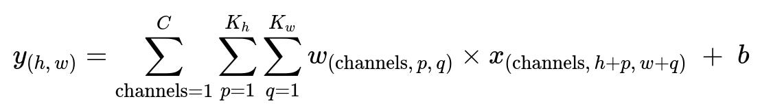
Here x is the multi-channel input feature map, w are the convolution filter weights, b is the bias term, and K_h, K_w represent the filter’s height and width. The result y_(h,w) is the output activation at spatial location (h,w).

When converting a Dense layer to a convolutional layer, one typically uses a 1x1 filter (or a kernel size matching the entire spatial dimension of the preceding layer’s feature map) with the number of filters corresponding to the number of outputs in the Dense layer. This 1x1 convolution effectively applies the same linear transformation that a Dense layer would, but it retains the spatial layout and can adapt to variable input sizes.

Key Steps for Conversion

One approach is to re-interpret the Dense layer’s weights as filters of size 1x1. The output dimension remains the same as the Dense layer’s output dimension, but instead of flattening the input, each 1x1 filter produces a single output channel. By stacking multiple 1x1 filters, you match the number of outputs needed. This operation can be repeated for multiple filters to replicate the fully connected behavior.

Concretely, if your Dense layer expects a flattened feature map of shape (C * H * W), you can reshape those weights into shape (out_features, C, 1, 1) in a convolution sense, provided that H * W is the prior flattening dimension. If H and W are the entire spatial dimensions of your feature map, you might replace them with a convolutional layer that has kernel_size=(H,W). This kernel size collapses the spatial dimension in a single pass, effectively doing the same matrix multiplication that the Dense layer would do, but in a convolutional manner.

Practical Implementation Details in PyTorch

import torch
import torch.nn as nn

class OriginalCNN(nn.Module):
    def __init__(self):
        super(OriginalCNN, self).__init__()
        self.features = nn.Sequential(
            nn.Conv2d(in_channels=3, out_channels=64, kernel_size=3, padding=1),
            nn.ReLU(),
            # other convolution or pooling layers
        )
        # Suppose we end up with a certain (C, H, W)
        self.classifier = nn.Sequential(
            nn.Flatten(),
            nn.Linear(in_features=64*7*7, out_features=100),
            nn.ReLU(),
            nn.Linear(in_features=100, out_features=10)
        )

    def forward(self, x):
        x = self.features(x)
        x = self.classifier(x)
        return x

class FullyConvCNN(nn.Module):
    def __init__(self):
        super(FullyConvCNN, self).__init__()
        self.features = nn.Sequential(
            nn.Conv2d(in_channels=3, out_channels=64, kernel_size=3, padding=1),
            nn.ReLU(),
            # same feature extraction
        )
        # Replace the linear layers with 1x1 convolutions
        self.conv_classifier = nn.Sequential(
            nn.Conv2d(in_channels=64, out_channels=100, kernel_size=7),
            nn.ReLU(),
            nn.Conv2d(in_channels=100, out_channels=10, kernel_size=1)
        )

    def forward(self, x):
        x = self.features(x)
        # Here we assume the feature map from self.features is 64 x 7 x 7
        x = self.conv_classifier(x)
        # If we want a final vector output (for classification), we can do:
        x = torch.squeeze(x)  # shape becomes [batch_size, 10]
        return x

In the FullyConvCNN, kernel_size=7 for the first convolution in the classifier block collapses the entire 7x7 spatial dimension, mimicking the effect of a Dense layer with in_features=6477. After that, a 1x1 convolution transitions from 100 channels to 10 channels, similar to the second Dense layer in the original network.

Why This Conversion Works

Flattening the output of the previous layers in a typical Dense layer discards the notion of spatial relationships. A fully convolutional approach preserves the spatial structure, allowing you to handle inputs of varying dimensions. This is particularly beneficial in tasks like segmentation, object detection, or any scenario where you want to maintain spatial correspondences through to the output layer.

Potential Follow-Up Questions

How do we handle mismatched shapes when converting a Dense layer to a convolution layer?

You can adjust the kernel_size or the stride and padding of the convolution so that the final output shape matches the intended dimensions. Ensuring that the number of input channels to the convolution matches the channel count of the preceding layer is also crucial. If the spatial dimensions do not match exactly, you might need a different kernel_size that covers the entire feature map, or you might need to add intermediate layers such as global average pooling to reduce the spatial dimension to 1x1 before applying a 1x1 convolution.

What are the advantages of a fully convolutional layer over a Dense layer in a CNN?

A fully convolutional layer can handle arbitrary input sizes because there is no need to flatten to a fixed-length vector. This can be especially useful in tasks that require per-pixel output, such as semantic segmentation, where each output pixel corresponds to some portion of the input. Additionally, fully convolutional networks preserve spatial information and can be more parameter-efficient in certain configurations.

How does training time compare when using Dense layers versus fully convolutional layers?

Training time and memory usage can vary depending on the specific architecture. When the spatial resolution is large, the fully convolutional layer might process bigger intermediate feature maps, leading to higher computational cost. However, if the architecture is designed carefully (e.g., reducing spatial dimensions via pooling or strided convolutions before applying 1x1 convolutions), the parameter count might be lower than a large Dense layer. In many practical cases, fully convolutional networks are highly efficient because you can maintain fewer total parameters while still exploiting large receptive fields through convolution.

Can we apply pre-trained weights from a Dense layer to the newly formed convolutional layer?

Yes, it is possible to reshape the pre-trained Dense layer’s weight matrix into the corresponding 1x1 convolutional filters, because they essentially represent the same shape of transformation (assuming you match the number of channels and the total input size). You would reshape the Dense layer’s weights from a shape of (out_features, in_features) into (out_features, in_channels, kernel_size_h, kernel_size_w), and do the same for the bias vector. This process is often done when converting classification networks (with Dense layers at the end) into fully convolutional networks for tasks like semantic segmentation.

When converting a Dense layer to a convolution layer, what issues arise with padding and stride?

In a fully convolutional layer, the stride and padding define how the filters traverse the input spatially. If you mimic the behavior of a Dense layer, you typically use stride=1 and no extra padding, with kernel_size matching the exact spatial dimension if you want a single output position for each output filter. Any deviation from these parameters will change the output’s spatial size or potentially shift the receptive field. Ensuring correct padding and stride is critical to preserve the expected alignment and size of the feature map.

Below are additional follow-up questions

Handling input images with widely varying sizes or aspect ratios

A fully convolutional layer can process variable-sized inputs by applying filter operations in a sliding window fashion. However, if the subsequent layers (such as pooling or strided convolutions) reduce the spatial dimensions aggressively, outputs might become too small or zero-dimensional for exceptionally small inputs. One practical way to handle this is to insert global pooling layers, which adaptively pool the spatial dimension into a fixed-size feature vector. For images with wide aspect ratios, you can also pad or crop them to standard sizes, though doing so might distort the image or discard information. A more robust alternative is to maintain the original aspect ratio through letterboxing (padding only in one dimension) and let the convolutional network handle the rest. Still, carefully monitoring how the aspect ratio affects the receptive field is key; in extreme aspect ratios, certain network structures might fail to capture essential context.

Potential dimension changes mid-network

In some architectures, the feature map size changes because of pooling, strides, or dilations. If you replace a Dense layer with a fully convolutional layer that expects a particular spatial dimension, any mismatch could cause shape errors or lead to unintended broadcasting. For example, a mid-network layer may produce an 8x8 feature map, but if you configure your convolutional replacement to have a kernel_size of (7,7), you might inadvertently alter the expected output if the input shape changes to 10x10 or 6x6 in a different data batch or model variation. A robust solution is to use adaptive pooling or carefully structure the network so that the spatial dimension before the fully convolutional layer is always well-defined (for instance, through standard repeated pooling operations). Another strategy is to dynamically infer the kernel size at runtime based on the current spatial shape, though this approach can complicate the weight-sharing assumption across different input shapes.

Potential numerical stability or initialization issues

When transitioning from Dense layers to their convolutional equivalents, the initialization scheme can have an impact on training stability. Dense layers often use initializations like Xavier or Kaiming uniform, which assume a certain distribution of inputs and outputs. Convolutions, though mathematically similar, may have a slightly different fan-in/fan-out depending on the kernel size. If you convert a Dense layer with shape (out_features, in_features) into a 1x1 convolution with shape (out_features, in_channels, 1, 1), you need to ensure that the in_features matches in_channels * the spatial area accounted for by the original flattening. A mismatch could lead to incorrect initialization scaling, which in turn might cause vanishing or exploding gradients. Ensuring the normalization layers (like BatchNorm) are correctly placed can also help stabilize training when using fully convolutional approaches.

Use beyond semantic segmentation

Although fully convolutional architectures gained popularity through segmentation tasks (where the goal is to predict labels for every pixel), they also find utility in other areas. For example, super-resolution networks often rely on fully convolutional structures to upscale images of arbitrary size. In object detection frameworks (like YOLO), the final layers are often fully convolutional to produce bounding box predictions for different regions without flattening. Another example is style transfer networks, which apply transformations to entire images. By removing Dense layers and operating entirely in a convolutional manner, these networks can handle images of various dimensions more naturally. This adaptability can simplify deployment when your application must handle diverse input shapes in real time.

Receptive field differences

Dense layers technically have a “global” receptive field because each neuron connects to every input element after flattening. Convolutional layers also achieve a global receptive field eventually, but they do so progressively through multiple stacked layers. The benefit of the fully convolutional approach is that you can trace back precisely how each output feature depends on localized regions in the input, which is valuable for interpretability and tasks like saliency maps. In scenarios requiring global context early in the network, you might consider skip connections or dilated convolutions that increase receptive field size without heavy parameter usage. Over-relying on large kernel sizes or repeated pooling can compromise fine-grained spatial details, so careful design is needed.

Strategies to reduce overfitting

When replacing Dense layers with fully convolutional layers, the number of parameters may still be large, and overfitting can be an issue. Common solutions include data augmentation (random crops, flips, rotations), regularization layers (such as Dropout placed after convolutional blocks), and weight decay in your optimizer settings. Dropout, however, behaves slightly differently in convolutional layers (where it might mask entire channels if applied in a channel-wise manner, as in SpatialDropout), so ensure the implementation aligns with your architecture’s requirements. Another strategy is to reduce the depth or number of filters in the fully convolutional part. This can maintain representational power while controlling parameter count.

Data augmentation

Data augmentation is typically applied to inputs, and fully convolutional networks benefit from the same set of augmentations as standard CNNs (e.g., random horizontal flip, random rotation, color jitter). A key subtlety arises if your task involves preserving exact spatial correspondences (e.g., segmentation masks or keypoints). In such cases, you must apply the same geometric transformations to both the input image and the corresponding label maps or annotations. Because the fully convolutional layers do not flatten the data, you can apply more region-specific or pixel-level augmentations (like random elastic deformations) while preserving the shape for direct pixel-wise comparisons in the output. The convolutional structure is inherently translation-invariant, so random translations or crops can help the model generalize better without losing the advantage of local receptive fields.

Performance considerations

While fully convolutional layers can handle arbitrary input sizes, the computational cost can become significant if the input feature maps remain large in intermediate stages. For example, if you remove a Dense layer that had a fixed input size and replace it with a convolution that operates on a much larger spatial dimension, your FLOPs (floating-point operations) could increase substantially. This is particularly notable if you keep the same number of filters. Techniques such as stride adjustments, dilations, or pooling can help reduce the resolution to a manageable level before applying the fully convolutional layer. Profiling tools in frameworks like PyTorch or TensorFlow can reveal bottlenecks, letting you optimize for speed or memory usage without significantly sacrificing model accuracy.

Managing final classification output shape for variable input

If you want a classification output (e.g., 10 classes) from a fully convolutional network but your input images can be of different sizes, you must reduce the feature map spatial dimension to 1x1 before you generate class logits. One approach is to use global average pooling across the spatial dimensions of the last convolutional feature map, resulting in a shape of (batch_size, num_channels). You can then apply a 1x1 convolution or a small fully convolutional layer to get the final class predictions. This strategy allows the network to operate on diverse input sizes. However, you should confirm that the global pooling does not discard crucial localization cues needed for accurate classification. Balancing the trade-off between preserving spatial features and obtaining a consistent output dimension is key.

Fully convolutional approach in object detection

In object detection, fully convolutional networks allow for efficient inference by treating detection as a dense prediction problem over a grid. Instead of having a Dense layer that outputs a fixed set of bounding box coordinates (which would require flattening), the network produces a tensor whose dimensions correspond to locations in the original image, with each location predicting objectness scores and bounding box offsets. This fully convolutional structure also simplifies dealing with different input image sizes—detections scale accordingly with the convolutional feature map. However, care is needed when choosing anchor sizes or feature map scales to ensure the network can detect objects at varying scales. Another subtle point is that if you rely on region proposals or multi-scale feature maps, you must design each block to remain fully convolutional to retain the benefit of flexible input dimensions.