ML Interview Q Series: What sets apart the two primary variations of Hierarchical Clustering approaches?

📚 Browse the full ML Interview series here.

Comprehensive Explanation

Hierarchical clustering is a class of clustering algorithms that seek to build a hierarchy of clusters. The main difference is whether we proceed in a bottom-up fashion (Agglomerative Hierarchical Clustering) or in a top-down manner (Divisive Hierarchical Clustering). Both rely on the concept of repeatedly merging or splitting clusters based on a measure of similarity or distance.

Agglomerative Hierarchical Clustering

In agglomerative clustering (sometimes called bottom-up approach):

• We begin with each individual data point as its own cluster.

• At each step, we merge two clusters that are most similar (or, equivalently, have the smallest distance).

• We continue this process iteratively until all data points end up in a single cluster.

A variety of linkage criteria can be used in this merging process:

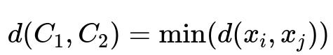
• Single linkage: The distance between two clusters is defined as the minimum distance between any member of one cluster and any member of the other. One can represent this central formula as:

  

  where x_i belongs to cluster C_1, and x_j belongs to cluster C_2. Here, d(x_i, x_j) is the distance between points x_i and x_j. The result is that the pairwise closest members of the two clusters define the distance between these clusters.

  • Complete linkage: Uses the maximum distance between points in each cluster.

  • Average linkage: Uses the average pairwise distance between points in the two clusters.

  • Ward’s linkage: Minimizes the variance within each cluster when merged.

  After merging clusters at each iteration, we typically use a dendrogram to visualize the progressive merging. By selecting a particular level in the dendrogram, we choose how many clusters to form.

  Divisive Hierarchical Clustering

  In divisive clustering (top-down approach):

  • We begin with all data points together in a single cluster.

  • In each step, we split one existing cluster into two subclusters.

  • We continue recursively splitting subclusters until each data point ends up in its own singleton cluster, or until we meet a stopping condition (like a specified number of clusters).

  Because it recursively partitions from a single group of all data points, divisive approaches can be conceptually more expensive. One might need to decide, at each stage, which cluster is the best candidate to be split, and how that split should be done (for instance, by using a standard clustering method like k-means to partition one cluster into two).

  Key Differences

  • Starting Point: Agglomerative begins with each point in its own cluster and merges upward; divisive starts with a single cluster and splits downward.

  • Computational Complexity: Agglomerative methods can be more straightforward to implement with known linkage criteria; divisive methods often require more computational effort, as each division might itself be a non-trivial clustering problem.

  • Practical Usage: Agglomerative hierarchical clustering is more commonly used in practice. Divisive methods can be useful in certain specialized cases or with specific domain knowledge on how to split clusters at each level.

  Example of Implementation in Python (Agglomerative)

  import numpy as np
  from sklearn.cluster import AgglomerativeClustering
  
  # Sample data
  X = np.array([
      [1, 2],
      [2, 3],
      [2, 2],
      [8, 7],
      [8, 8],
      [25, 80]
  ])
  
  # Agglomerative Clustering
  agg_cluster = AgglomerativeClustering(n_clusters=2, linkage='single')
  labels = agg_cluster.fit_predict(X)
  print("Labels from Agglomerative (Single Linkage):", labels)
  

  In this snippet, we are performing agglomerative clustering with a single-linkage criterion. The fit_predict method returns the cluster labels for each data point.

Practical Considerations

Choosing between agglomerative and divisive may depend on:

• Size of the dataset: For very large datasets, certain hierarchical strategies might be computationally intensive. Approximate methods or truncated dendrogram approaches may be needed.

• Desired granularity: Being able to visualize the dendrogram in agglomerative clustering can help in deciding how many clusters to form. Divisive methods are sometimes more interpretable if you have a strong notion of how to progressively break down the data.

• Linkage criteria and distance: Different linkage criteria can yield different cluster shapes and structures. For example, single linkage can produce chain-like clusters; complete linkage tends to form more compact clusters.

Potential Follow-Up Questions

How do you decide the number of clusters in hierarchical clustering?

In a real-world scenario, the number of clusters may not be known in advance. A common approach is to:

• Look at the dendrogram and find a “significant jump” in the distance between merges. A larger jump near a certain level indicates that merging beyond this point would group fairly dissimilar clusters into one.

• Use cluster validity indices such as the Silhouette Score or the Dunn Index to evaluate different cut points along the dendrogram.

Additionally, domain knowledge can guide where to “cut” the dendrogram based on meaningful distinctions in the data.

Could you describe some edge cases or pitfalls in hierarchical clustering?

Some edge cases and pitfalls include:

• Sensitivity to Noise: If outliers exist, certain linkage criteria (e.g., single linkage) can produce undesirable “chaining effects,” where outliers cause clusters to merge earlier than expected.

• Computational Complexity: For extremely large datasets, building and updating a distance matrix can be expensive (often O(n^2) or worse). Approximation or partial clustering methods might be needed.

• Linkage Choice: Different linkage metrics can lead to drastically different results. It is important to experiment with multiple linkage strategies or rely on domain knowledge to pick the most appropriate one.

• Scaling: The distance metric used can significantly affect the clustering outcome, so it is crucial to normalize or scale features appropriately if they are on different numeric ranges.

How does Ward’s linkage differ from other linkage criteria?

Ward’s linkage approach focuses on minimizing the increase in the sum of squared errors within clusters when two clusters merge. This often leads to more compact, spherical clusters in Euclidean space. It is beneficial when you want to preserve homogeneous groupings and control within-cluster variance. However, it tends to be more computationally intensive than simpler linkage metrics like single or complete linkage.

Can hierarchical clustering handle high-dimensional data effectively?

Hierarchical clustering can become less effective when dimensionality increases, due to the curse of dimensionality. Distances between points can become less meaningful in very high-dimensional spaces. Strategies include:

• Dimensionality Reduction: Techniques such as PCA, t-SNE, or UMAP can help reduce data dimensionality before clustering.

• Feature Selection: Carefully selecting relevant features can limit noise and improve cluster separability.

• Approximate Methods: For large, high-dimensional data, approximate nearest-neighbor search or sampling-based methods might be needed to keep computations tractable.

Are there any memory constraints to worry about when using hierarchical clustering?

Yes. Hierarchical clustering often requires storing a distance matrix of size n x n, which can be large for datasets with many instances. This memory complexity can become a bottleneck. Incremental and memory-efficient variants or partial clustering methods might be required for massive datasets.

By understanding the two forms of hierarchical clustering (agglomerative vs. divisive) along with their computational and practical differences, one can select the most suitable method based on data size, domain knowledge, and desired output structure.