ML Interview Q Series: What type of Cost Functions do Greedy Splitting use?

📚 Browse the full ML Interview series here.

Comprehensive Explanation

Greedy splitting in decision tree algorithms refers to the process of selecting a feature split (and the corresponding threshold in the case of continuous features) that maximizes some criterion at each node of the tree. The quality or “goodness” of a split is usually measured by how well it separates the target variable based on the chosen feature. The cost function indicates how “impure” the node is or how dissimilar the data points in that node are with respect to the target variable. By reducing impurity (or cost) in the children nodes, the decision tree ideally becomes more predictive.

When dealing with classification trees, the most commonly used cost functions for greedy splitting are Gini Impurity and Entropy (used in Information Gain). For regression trees, the most commonly used cost function is Mean Squared Error (MSE), or sometimes Mean Absolute Error (MAE). The goal in all cases is to pick splits that minimize the impurity or variance in the resulting partitions.

Classification Cost Functions

Entropy and Information Gain

Entropy measures the impurity in a classification context. A node with purely one class has zero entropy. If a node has multiple classes in relatively equal proportions, then it has high entropy. Decision tree algorithms like ID3 and C4.5 use Information Gain, which is computed from entropy differences before and after splitting.

In this expression, p_i is the fraction of elements in S (the node’s sample set) belonging to class i. When you split the node S into subsets S_left and S_right (for example), you measure the weighted sum of their entropies. The difference between the original node’s entropy and the weighted sum of entropies in the children is your Information Gain. A split that produces children with lower entropy (i.e., more pure subgroups) yields higher Information Gain.

Gini Impurity

The CART algorithm often uses the Gini Impurity. It tends to measure misclassification levels if a class is randomly assigned based on distribution in the node. Nodes dominated by one class will have a small Gini Impurity, while nodes with many classes in more balanced proportions will have a higher Gini Impurity.

Here, p_i represents the fraction of data points in class i within the node. If a node is predominantly of one class, then p_i will be close to 1 for that class, making the sum p_i^2 large and thus G small.

Regression Cost Function

In regression trees, the cost function is typically the variance of the target values in a node. Minimizing variance is often done by minimizing Mean Squared Error:

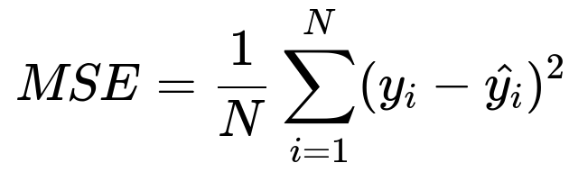
In this formula, y_i represents the actual target value for the i-th sample in the node, and \hat{y_i} is the predicted value (often the average of the target values in that node). N is the total number of samples in that node. During greedy splitting in regression trees, the objective is to find a partition that yields the largest drop in MSE (or variance) from the parent node to its children nodes.

Implementation Example in Python

Below is a sketch for how one might compute these measures. This example shows how to compute Gini Impurity and Entropy for a classification node, though in practice frameworks like scikit-learn or XGBoost handle these calculations internally.

import numpy as np
from collections import Counter

def gini_impurity(labels):
    # labels is a list or array of class labels in the node
    total_count = len(labels)
    if total_count == 0:
        return 0
    class_counts = Counter(labels)
    impurity = 1
    for class_label, count in class_counts.items():
        p = count / total_count
        impurity -= p**2
    return impurity

def entropy(labels):
    total_count = len(labels)
    if total_count == 0:
        return 0
    class_counts = Counter(labels)
    ent = 0
    for class_label, count in class_counts.items():
        p = count / total_count
        ent -= p * np.log2(p)
    return ent

def mse(values):
    # values is a list or array of numeric target values in the node
    if len(values) == 0:
        return 0
    mean_val = np.mean(values)
    return np.mean((values - mean_val)**2)

Whenever you split a set of data points into subsets, you can calculate each child's impurity (Gini or Entropy in classification or MSE in regression) and combine these with weights based on the number of samples in each subset. The split that achieves the highest reduction in impurity or variance is chosen.

Why Different Cost Functions?

In classification, Gini Impurity and Entropy often produce similar results in practice. The difference usually appears in how splits are prioritized: Gini tends to isolate the most frequent class first, whereas Entropy (Information Gain) emphasizes separation of all classes more uniformly. For regression tasks, MSE or variance-based splitting is a natural choice to capture how spread out the target values are.

Follow-up Questions

How does the choice between Gini Impurity and Entropy affect the final decision tree?

They usually produce very similar trees. Gini Impurity might be slightly faster to compute due to the absence of a logarithm in the formula. Entropy, on the other hand, captures more granular differences in class probabilities. In certain edge cases (like highly imbalanced classes), careful tuning and understanding of these subtleties can affect model performance. However, practical results often show negligible differences unless you have a specific reason to choose one over the other, such as interpretability or slight performance advantages.

Can we use cost functions other than MSE for regression splitting?

Yes, Mean Absolute Error (MAE) is sometimes used, especially when the distribution of residuals is heavy-tailed or you want to reduce the impact of outliers. Another cost function is Huber loss, which transitions from MAE to MSE depending on the magnitude of errors. Each of these can be used in a greedy splitting framework, although the computations may become more intricate.

Why do we call it a “greedy” approach?

The process is considered greedy because at each node you make the optimal split decision based solely on the current node’s impurity reduction, without regard for how this choice might affect future splits. This local optimization at each step can sometimes lead to suboptimal global trees. Pruning and ensemble methods (like Random Forests or Gradient Boosted Trees) can help mitigate potential overfitting or poor splits arising from this greedy strategy.

What happens if a tree keeps splitting until it perfectly classifies or predicts the training data?

You risk overfitting: the tree can grow to a size where each leaf (or most leaves) holds very few samples, possibly just one in the extreme. This will lead to poor generalization. Regularization techniques like limiting the maximum depth, setting a minimum number of samples per leaf, or pruning the tree after it’s grown are widely used to control overfitting.

How can one evaluate the final chosen splitting criterion?

Common approaches include cross-validation to compare performance metrics like accuracy or F1-score in classification, or mean squared error or R-squared for regression. If the chosen criterion (e.g., Gini vs. Entropy) consistently yields better performance on validation data for the problem at hand, it might be the right choice. However, the differences are often minimal, so it typically comes down to practical concerns such as computational efficiency and ease of interpretation.

All these considerations underscore that greedy splitting uses cost functions like Gini Impurity, Entropy (Information Gain), or MSE (variance reduction) to drive the construction of decision trees. Each is formulated to reduce impurity or variance locally at each node, leading to an overall tree that attempts to separate classes or predict numeric values effectively.

Below are additional follow-up questions

How do these cost functions handle multi-class classification?

Traditional cost functions like Gini Impurity and Entropy extend naturally to multi-class problems. In Gini Impurity, you simply sum up the squared probabilities of all classes that appear in a node. Similarly, with Entropy, you sum over all classes, multiplying their probability by the log of that probability.

In real-world multi-class scenarios, one subtlety is the distribution of classes. If some classes have very few examples, it’s possible for splits to appear optimal when mostly separating out the majority classes, while minor classes remain mixed. One potential pitfall is that a decision tree might not effectively isolate these minority classes. If your business problem values the smaller classes, consider additional methods such as class-weighting, or ensure your dataset is balanced enough.

When the number of classes grows large, the cost function computations become more intensive (since you must compute probabilities for each class). For most datasets this overhead is small, but with extremely large label spaces (like in certain NLP tasks), you might need to optimize or approximate the calculations. Nonetheless, the principle of summing probabilities remains unchanged.

Are there cost functions specifically tailored for imbalanced datasets?

Several techniques address the challenge of imbalanced datasets, even though Gini Impurity and Entropy remain standard. One approach is to modify these cost functions by incorporating class weights. For example, the weighted Gini Impurity would multiply p_i^2 by the class weight of class i, giving greater penalty for misclassifying a minority class.

Another approach is to use a different metric altogether, such as the Focal Loss (popularized in object detection tasks). While it is typically associated with neural networks, you can conceptually adapt it for splitting decisions in a decision tree. However, this tends to be non-trivial because decision trees are built around impurity-reduction in node subsets rather than direct gradient-based optimization.

Pitfalls include over-correcting for minority classes, which might lead to an overly large number of splits focusing on a small subset of data. This can heighten the risk of overfitting for rare classes. Class weighting or sampling techniques (like SMOTE) often help, but must be tuned carefully.

What is the role of the splitting threshold for continuous features, and how is it determined?

For a continuous feature, the greedy algorithm typically sorts the unique feature values and then tries potential thresholds between successive unique values. For instance, if you have a feature x with sorted unique values [2, 5, 5.3, 6.1], then candidate thresholds might be midpoints like 3.5, 5.15, or 5.7. For each threshold, the data is split into two subsets (<= threshold and > threshold), and the resulting cost function (Gini, Entropy, or MSE) is evaluated.

A subtlety here is that sorting the data and scanning over all possible midpoints can be computationally expensive when the dataset is large or features are high-dimensional. Some implementations use approximate methods to reduce computational costs, especially in gradient boosting frameworks that handle big data. Another pitfall is if a continuous feature has a large number of repeated values. The “unique values” might be fewer than the raw data points, but if you still have many unique values, scanning them all can be slow. Approximations or subsampling thresholds can mitigate this at the risk of missing the absolute best split.

Could we use cost functions from other domains, such as cross-entropy loss, for regression tasks?

Cross-entropy is typically associated with classification. In regression tasks, you are predicting continuous values, so cross-entropy is not directly applicable in the same sense. However, if you discretize the output space, you could theoretically transform a regression task into a classification-like problem with bins representing ranges of the target variable and then use cross-entropy to measure how well you separate those bins.

A key pitfall is that binning continuous data may destroy critical fine-grained variations in the target. You might also face the problem that many bins are empty or underpopulated, especially if the data distribution has long tails. In practice, MSE, MAE, or Huber loss is usually more stable and computationally straightforward for regression within a decision tree. Converting regression to classification with cross-entropy may be viable for specialized tasks, but it’s generally not standard for greedy splitting.

In practice, how do we handle missing values during greedy splitting?

Several strategies exist for handling missing values:

1. Ignore missing values during split computation: This might skew the impurity calculation if the data with missing values is not representative, or if missingness correlates with the target variable.

2. Imputation: Fill in missing values with the mean/median (for regression) or the most frequent class (for classification). However, this can introduce bias if the mechanism of missingness is non-random.

3. Separate branch for missing: Some implementations allow a split to have a branch that corresponds specifically to missing values. This can handle structured missingness patterns more elegantly, though it complicates the tree structure.

A subtle pitfall is that if missingness itself is informative (for instance, a missing value on a medical test could imply something about a patient’s condition), ignoring or naively imputing might degrade performance. Decision trees can sometimes glean extra signal by separating out those missing records. Another pitfall is that if the missingness is random, adding a separate branch might lead to overfitting on spurious patterns.

How do decision trees handle non-monotonic relationships with greedy splitting?

Decision trees are quite flexible in modeling non-monotonic relationships because each split is a local partition in the feature space. The tree can branch in ways that capture complex patterns, such as U-shaped or wave-like relationships, simply by creating multiple splits along that feature.

However, a big pitfall is that pure greedy splitting can require many splits to approximate strongly non-monotonic relationships, especially if the pattern is subtle or if there are multiple interacting features. This may lead to very deep trees that risk overfitting. Regularization methods like max_depth, min_samples_leaf, and pruning become particularly important in these cases. Without proper constraints, the model might create unnecessary splits that reduce impurity a small amount at each step but degrade generalization.

Is there a scenario where using misclassification error rate as the splitting criterion is more beneficial than Gini or Entropy?

Misclassification error rate for a node is 1 - max_class_probability. While this measure is simpler to interpret, it is not as sensitive to changes in the class distribution as Gini or Entropy. As a result, you may find that using misclassification error rate can yield shallower trees, because many potential splits produce similar improvements when measured by a less granular criterion.

A scenario where it might be beneficial is when interpretability is paramount and you want to limit the complexity of the tree. Misclassification error sometimes yields simpler splits that can be more easily explained. Additionally, if you only care about final classification accuracy without regard to class probabilities, misclassification error may suffice. However, a subtlety here is that Gini and Entropy can detect finer distinctions in how balanced the child nodes are, often leading to splits that overall yield better performance.

What are potential pitfalls when using MSE for large-scale regression tasks?

In large-scale settings with millions or billions of samples, computing MSE-based splits can be expensive because you need to recalculate means and partial sums repeatedly. Distributing or parallelizing the computation of MSE is possible, but if not done efficiently, it can become a bottleneck. Approximate or histogram-based strategies that bin the feature values are used in some implementations (e.g., in gradient boosting libraries) to speed up finding the optimal split threshold.

Another pitfall is that MSE can be highly sensitive to outliers. In massive datasets, even a relatively small cluster of extreme values can affect the mean significantly, and thus the chosen splits might cater excessively to these outliers. One real-world issue is that if your target variable includes extreme high or low values that are data errors or rare events, the tree might produce splits that are overfitted. Some practitioners switch to robust cost functions like MAE or the Huber loss in these cases, though that can increase computational complexity.

How does standard deviation reduction differ from MSE-based splitting?

The variance of a node’s target values is the squared standard deviation multiplied by (N-1)/N. Minimizing variance is equivalent to minimizing MSE in the node, because both measure the spread of values around the mean. In practice, many textbooks and frameworks mention “variance reduction” or MSE interchangeably when describing regression tree splitting.

A subtle difference arises in constants or scaling factors. MSE is an average measure: sum of squared errors divided by N. Variance is the sum of squared deviations from the mean divided by N or N-1 (depending on the definition). When choosing splits, the difference is typically just a constant factor that does not affect which split yields the greatest reduction. So from a decision-making standpoint, MSE-based splitting and standard deviation reduction lead to the same outcome. However, if a specific library uses an unbiased variance estimate dividing by (N-1), that is a minor difference in implementation details rather than conceptual approach.