

📚 Browse the full ML Interview series here.
Comprehensive Explanation
Covariance and Correlation measure how two variables move together, but they do so at different scales. Covariance can be interpreted as a measure of the joint variability of two random variables. Correlation, on the other hand, is a standardized form of covariance, ensuring its values always lie between -1 and +1. The main conceptual difference is that covariance describes the direction of linear relationships but is still affected by the units of measurement. Correlation removes the effect of scale by normalizing covariance with the product of standard deviations.
Mathematical Definitions
Covariance is defined as the expected value of the product of the deviations of X and Y from their respective means. The core formula for covariance is shown below.
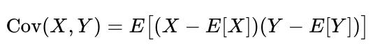
In this expression, X and Y are random variables, E[X] is the mean of X, and E[Y] is the mean of Y. The measure Cov(X, Y) can be positive or negative. A positive value means that when X is above its mean, Y tends to be above its mean as well, and vice versa.
Correlation is the normalized measure of covariance, defined by dividing the covariance by the product of the standard deviations of X and Y.

Here, sigma_X is the standard deviation of X, and sigma_Y is the standard deviation of Y. As a result of this normalization, correlation values range from -1 to +1, which makes them easier to interpret and compare across different datasets. Correlation focuses on the strength and direction of a linear relationship, irrespective of the absolute scales of X and Y.
Practical Interpretation
Covariance alone can be difficult to interpret because its value depends on the scales of the variables. If you scale your data by a constant factor, the covariance changes, making direct comparisons tricky. Correlation, being dimensionless, allows you to compare relationships across different problems and scales. If you want a measure of how closely two variables are related in a linear sense (and in a way that is not influenced by varying scales), you typically use correlation.
Python Implementation Example
Below is a small Python snippet to illustrate how one might compute covariance and correlation using libraries like NumPy. Note that these functions are usually readily available in libraries such as pandas or NumPy, but this is a straightforward implementation.
import numpy as np

# Example data
X = np.array([1.5, 2.3, 3.1, 4.0, 5.2])
Y = np.array([2.0, 2.5, 3.7, 3.8, 5.0])

# Manual computation of covariance
mean_X = np.mean(X)
mean_Y = np.mean(Y)
covariance = np.mean((X - mean_X) * (Y - mean_Y))

# Manual computation of correlation
std_X = np.std(X)
std_Y = np.std(Y)
correlation = covariance / (std_X * std_Y)

print("Covariance:", covariance)
print("Correlation:", correlation)
This code calculates covariance by taking the average of (X - mean_X)(Y - mean_Y) and then normalizes by multiplying by 1/(sigma_Xsigma_Y) for correlation. In practice, you can also use np.cov(X, Y)[0,1] for covariance and np.corrcoef(X, Y)[0,1] for correlation.
Why We Need Both Covariance and Correlation
Covariance is helpful when the scale of the variables is meaningful, especially in certain fields such as finance, where you might be interested in how the magnitude of one variable affects another. However, correlation is more commonly used for quickly assessing linear relationships in a way that is comparable across different problems. Correlation values are dimensionless, which is particularly useful when combining or comparing results across datasets with varying units.
Potential Follow-up Questions
What does a negative correlation imply, and how does it differ from negative covariance?
A negative correlation implies that as one variable increases relative to its mean, the other variable tends to decrease relative to its mean, and vice versa. In terms of negative covariance, it means the product (X - E[X])*(Y - E[Y]) is on average negative. Because correlation is normalized, a negative correlation near -1 signifies a strong, perfectly inverse linear relationship, whereas a covariance could be negative yet small or large depending on the scales of the variables.
If correlation is zero, does it mean there is no relationship between the variables?
A correlation of zero only means there is no linear relationship. The variables could still be related in non-linear ways. Covariance and correlation focus strictly on linear patterns. There may be more complex relationships (for instance, quadratic or other non-linear forms) that neither covariance nor correlation fully captures.
How would you interpret correlation or covariance in high-dimensional data?
In high-dimensional data, interpreting pairwise correlation or covariance can be tricky because multiple variables can interact in complex ways. One has to be cautious about spurious correlations. Techniques like regularization, dimensionality reduction, or partial correlation (conditioning on other variables) might be necessary to isolate meaningful relationships. Covariance matrices in very high dimensions can become ill-conditioned, so special care is needed, such as shrinkage estimators.
When might you prefer to use covariance instead of correlation?
You might prefer covariance in contexts where you care about the raw scale of how two variables move together. In finance, for instance, portfolio variance is computed using covariances. The actual magnitude of Cov(X, Y) can matter if you want to assess how a change in one variable might predict the scale of changes in another variable. If you only want a measure of linear association without units, correlation is the standard choice.
Are covariance and correlation robust to outliers?
Covariance and correlation are based on means and standard deviations, so they are not robust to outliers. A single extreme value can significantly affect both. If a dataset has heavy-tailed distributions or potential for extreme values, more robust measures (for example, Spearman's rank correlation for correlations or other robust estimators for covariance) might be more appropriate.
What could cause correlation values to be misleading?
Correlation may be misleading if the data have significant non-linear patterns, outliers, or if subsets of data differ in scale or distribution. Another classic pitfall is Simpson’s paradox, where a trend apparent in different groups of data disappears or reverses when these groups are combined. Always inspect data visually (e.g., scatter plots) to confirm any correlation or covariance findings.
How do you handle correlation in a machine learning pipeline?
In feature selection or dimensionality reduction, you often look at correlations to identify redundant features. Highly correlated features may not both be needed. But because correlation is only a measure of linear association, it cannot detect certain non-linear dependencies. Therefore, you might supplement correlation checks with mutual information or other methods to detect more general relationships.
By understanding both covariance and correlation in detail, you can better decide which measure is most relevant for a particular machine learning or statistical problem, and you can diagnose potential pitfalls in data analysis and model building.
Below are additional follow-up questions
How can correlation be spurious, and what steps would you take to detect or prevent it?
Spurious correlation can arise when two variables appear to have a strong linear association but in reality are driven by a third, hidden factor or by purely coincidental patterns. A classic example is a strong correlation between global ice cream sales and the number of shark attacks, both driven by warmer weather (a third variable), not by a causal link between ice cream consumption and shark aggression.
To detect or prevent spurious correlation, it helps to examine potential confounding variables and to see if they are responsible for the observed relationship. This can involve partial correlation, where you control for the effect of a third variable, or more sophisticated methods such as regression-based analyses that include additional relevant features. It is also useful to segment the data and see if the correlation remains consistent within different subsets. If the correlation vanishes or reverses in these subsets, that suggests an external factor is at play.
When working with large datasets, it is common to find statistically significant correlations by chance. In such scenarios, correcting for multiple hypotheses testing (for example, the Bonferroni correction or False Discovery Rate adjustments) is often necessary to reduce the risk of spurious findings.
Real-world pitfalls include:
Confounding variables that inflate or hide true relationships.
Coincidental correlations that are statistically significant but have no real-world meaning.
Data mining large feature sets without proper significance corrections.
What is the difference between correlation and cross-correlation in time series analysis?
Correlation typically measures how two variables co-move without an explicit notion of time-lag. Cross-correlation, however, is specifically used in time series contexts to detect potential lead-lag relationships. Instead of aligning the data by identical time indices, you shift one time series in increments (lags) and measure how well it lines up with the other. This process indicates whether changes in one variable precede changes in the other at some delay.
This difference can significantly alter the interpretation. A standard correlation might show no strong relationship if you compare variables at the same time point, but cross-correlation can reveal a strong association when one series is time-lagged by some interval. If cross-correlation at lag k is significantly high, it suggests that events in the first series can help predict events in the second series k time units in the future.
Potential pitfalls include:
Overlooking underlying seasonality or trends that inflate cross-correlation.
Misinterpreting correlation at a certain lag as causation without further context or domain knowledge.
Not properly differentiating non-stationary time series before performing cross-correlation.
How do you handle missing data when measuring correlation or covariance?
Missing data can distort both covariance and correlation if not addressed properly. Common approaches include listwise (complete case) deletion, pairwise deletion, or imputation.
Listwise deletion drops any row in which any variable is missing, reducing the dataset’s size and risking bias if the data are not Missing Completely at Random (MCAR).
Pairwise deletion uses all available data for each pair of variables, which can yield more data points than listwise deletion but can complicate interpretation because the sample size for each pair differs.
Imputation techniques fill in missing values, for example, with mean imputation, or more advanced methods like multiple imputation or model-based approaches. These methods can be helpful but rely on assumptions about the missingness mechanism. Poorly chosen imputation methods can skew correlations.
In practical settings, verifying that the data are MCAR or Missing at Random (MAR) is crucial. If they are Missing Not at Random (MNAR), results from any standard correlation or covariance measure might be heavily biased. Sensitivity analysis is often done to see how different assumptions about the missingness mechanism affect the results.
What is the effect of strong leverage points or extreme values on covariance and correlation?
Leverage points refer to data instances in the predictor space that are far from the average, potentially exerting a disproportionate influence on fitted models. Extreme values (outliers) in either variable can dramatically inflate or deflate covariance and correlation because both measures depend on the mean and standard deviation.
An outlier in one variable might cause an artificially high or low product (X - mean_X)*(Y - mean_Y), affecting covariance directly. Because correlation normalizes by the product of standard deviations, an outlier can also inflate these standard deviations in a way that obscures or distorts the real relationship.
To diagnose such issues:
Visual inspection via scatter plots to identify potential outliers.
Use robust correlation measures, such as Spearman’s or Kendall’s tau, for non-parametric correlation that reduces sensitivity to extreme values.
Apply robust estimators of covariance (e.g., Minimum Covariance Determinant) if outliers are expected.
How does correlation factor into portfolio optimization in finance, and can we rely on it for risk diversification?
In finance, portfolio optimization, particularly under the Modern Portfolio Theory framework, relies on the covariance matrix to determine risk (variance) and to find an optimal distribution of assets. Correlation often provides a simplified lens: If two assets have a low or negative correlation, their combined portfolio risk is typically lower when held together, assuming returns remain constant.
However, correlation in financial markets can be dynamic. Low or negative correlations under “normal” market conditions can spike towards 1 in times of crisis, a phenomenon known as correlation breakdown. This undercuts the expected diversification benefit right when it is most needed.
Risk management teams often look at rolling correlations or stress-test correlations under specific scenarios. They may also model correlation asymmetry, recognizing that correlations can change during volatile periods. Reliance solely on historical correlation can create a false sense of security if future market conditions differ greatly from the past.
How is correlation used in dimensionality reduction techniques like PCA, and does covariance play a different role?
Principal Component Analysis (PCA) can be performed on either the covariance matrix or the correlation matrix, each serving slightly different purposes:
When PCA uses the covariance matrix, it preserves the scale of each original variable. This is often suitable if you believe that the scale holds meaningful information.
When PCA uses the correlation matrix, each variable is first standardized (mean=0, variance=1). This approach is beneficial when variables have vastly different units or scales and you want to treat them equally in the analysis.
Mathematically, PCA on the correlation matrix is the same as running PCA on the standardized data’s covariance matrix. Covariance-based PCA might be skewed by a single variable with large variance, while correlation-based PCA ensures every variable contributes equally at the outset. The choice depends on whether preserving the original scale is vital or not.
If two variables have a correlation of +1, does that imply they share the exact same distribution?
A correlation of +1 indicates a perfect linear relationship: one variable can be expressed as a linear transformation of the other. That is, Y = aX + b with a > 0. However, having exactly the same distribution requires more than just a perfect linear relationship. If a is not 1, then the variance of Y differs from that of X; similarly, if b is not 0, the means differ.
Even though they move together linearly, the distributions might differ in location and scale. Perfect correlation does guarantee a deterministic linear mapping, but not identical distribution moments (unless a=1 and b=0). Also, correlation does not capture higher moments such as skewness or kurtosis, so two perfectly correlated variables can still differ in those respects if one is a linear shift or scale of the other.