
ML Interview Q Series: When designing a deep neural network, what are the key considerations to keep in mind while picking a suitable loss function?

📚 Browse the full ML Interview series here.
Comprehensive Explanation
Choosing an appropriate loss function is crucial because it directly influences how the model parameters are updated during training. The loss function quantifies the discrepancy between the model’s predictions and the true target values, guiding gradient-based optimization. The selection of a loss function typically depends on factors like the type of task (regression vs. classification vs. generative modeling), data distribution, presence of outliers, and practical deployment constraints.
Common Loss Functions
Mean Squared Error (MSE) for Regression
MSE is widely used for regression tasks where the goal is to predict continuous values. It penalizes large errors more than small ones due to the squaring of the residual.
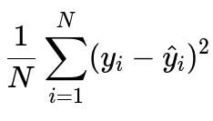
where y_i is the ground truth continuous value for the i-th sample, and \hat{y}_i is the model's predicted value for the i-th sample. N is the total number of samples in the dataset.
MSE provides a convenient, smooth surface for gradient-based methods, and it is symmetric around zero. However, it is sensitive to outliers because any large deviation gets squared and can disproportionately affect parameter updates.
Cross-Entropy for Classification
Cross-Entropy (also referred to as log loss) is a standard choice for classification problems. It measures the difference between two probability distributions: the predicted probabilities and the true distribution (often represented as a one-hot vector in the case of multi-class classification).

where y_i is the true label for the i-th sample (for binary classification typically 0 or 1), and \hat{y}_i is the predicted probability for the positive class. N is the total number of samples.
Cross-Entropy loss encourages the model to output probabilities close to 0 or 1, thus becoming a powerful metric when the final output must be a valid probability. Extensions such as categorical cross-entropy or multi-label variants exist for multi-class or multi-label problems.
Other Loss Functions
In some situations, specialized loss functions may be necessary:
Huber loss, which is less sensitive to outliers than MSE and is often used for robust regression.
L1 loss (Mean Absolute Error), which can produce more robust estimates to outliers but might lead to non-differentiability at 0.
Dice loss or IoU-based losses for segmentation tasks in computer vision, especially for imbalanced segmentation classes.
Kullback–Leibler divergence or other distribution-based losses in generative modeling.
Influencing Factors
Data Distribution and Outliers
If the dataset has heavy-tailed distributions or many outliers, MSE can be problematic. Losses like L1 or Huber loss can limit the influence of outliers. For classification tasks with skewed class distributions, cross-entropy alone may not be enough; you might consider weighting the loss to handle class imbalance.
Model Output Type
If the network outputs probabilities, a probabilistic loss (like cross-entropy) aligns well with that design. If the network outputs unconstrained continuous variables, typical regression losses (like MSE or L1) are more appropriate.
Practical Training Stability
Loss functions with smooth gradients tend to stabilize training. Sudden large gradients (as can arise in certain custom or piecewise-defined losses) may require specialized optimizers or careful tuning of the learning rate.
Domain Requirements
There might be domain-specific objectives that standard losses do not capture. For example, in ranking or recommendation, one might use a ranking loss (e.g., pairwise ranking loss). In image-to-image tasks, perceptual losses (using features from pretrained networks) sometimes better match the subjective quality desired.
How to Handle Imbalanced Data with the Chosen Loss Function?
In scenarios where the dataset has significantly more examples of one class than another, standard cross-entropy may underweight rare classes. One approach is to use class weighting, where you increase the penalty for misclassifying underrepresented classes. Another technique is focal loss, which down-weights well-classified samples so the model focuses more on the harder, misclassified examples. The right choice depends on the severity of the imbalance and the performance metric (e.g., F1 score, precision, recall) you aim to optimize.
Strategies for Multi-Label Classification
When each sample can belong to multiple classes simultaneously, binary cross-entropy is often applied to each class independently, assuming independence among the labels. If the labels are correlated, more sophisticated losses that account for label dependencies might be used (for example, a structured prediction approach). You can also adapt weighting strategies to multi-label settings to deal with class imbalance.
Interpreting Gradients and Optimization Dynamics
The chosen loss function affects the gradient magnitude and direction. For instance, MSE tends to produce smaller gradients when errors are small, which can slow learning if the model is near a local minimum. Cross-entropy typically generates larger gradients even when predictions are close to the target, potentially accelerating convergence. Understanding these dynamics helps in diagnosing training issues such as vanishing or exploding gradients.
Impact of Multi-Modal Output Distributions
If the target output can have multiple valid modes (e.g., a trajectory that could proceed in multiple equally valid ways), a single unimodal loss like MSE might not capture the distribution well. In these cases, mixture density networks or other probabilistic techniques can model multi-modal outputs by optimizing a likelihood-based loss (like a Gaussian mixture negative log-likelihood). The loss choice should align with the true data distribution if the model needs to capture multiple plausible outcomes.
Adjusting the Loss for Shifting Data Distributions
When the real-world data distribution changes over time (concept drift), a static loss function may lose relevance. One might incorporate adaptive weighting that periodically recalculates the importance of certain classes or certain types of mistakes. Monitoring performance metrics on a validation set in real-time can provide signals to update or re-weigh the loss function accordingly.
Practical Implementation Examples
import torch
import torch.nn as nn
import torch.optim as optim

# Example for a binary classification model
model = ...  # Some neural network architecture
criterion = nn.BCELoss()  # Binary cross entropy
optimizer = optim.Adam(model.parameters(), lr=0.001)

for data, labels in dataloader:
    optimizer.zero_grad()
    outputs = model(data)
    loss = criterion(outputs, labels)
    loss.backward()
    optimizer.step()

# Weighted cross-entropy for imbalanced classification
weights = torch.tensor([0.25, 0.75])  # Example: weight minority class more
weighted_criterion = nn.CrossEntropyLoss(weight=weights)
In the above snippet, binary cross-entropy is used for a binary classification task. For tasks with imbalance, weighting the classes (or using specialized losses like focal loss) helps.
Important Edge Cases and Pitfalls
Using a non-smooth loss function can cause optimization instabilities or require special optimization techniques. Also, an inappropriate choice can cause model overconfidence (e.g., cross-entropy with high class imbalance might push the model to focus on the majority class only). In real-world scenarios, it is also vital to validate the alignment between training loss and the business metric of interest—sometimes, a specialized metric might be better optimized by a custom or surrogate loss.
How to Choose the Best Loss in Practice?
One pragmatic approach is to start with conventional choices (MSE for regression, cross-entropy for classification) and then evaluate performance on validation or test sets. Based on error analysis, you might introduce modifications (such as weighting or custom penalty terms) that capture the nuances of your data distribution or application requirements. Experimenting with domain-specific losses and systematically analyzing results often yields the most effective configuration for real-world tasks.
Below are additional follow-up questions
What if the Data Contains Highly Noisy or Incorrect Labels?
In real-world scenarios, labels might be unreliable or noisy. When labels are wrong or randomly assigned, the training signal can be misleading. This problem appears frequently in crowdsourced datasets, sensor data subject to calibration issues, or large-scale web-scraped text/image data. An inappropriate loss function can overfit these flawed labels, harming generalization.
A possible solution is to adopt robust loss functions (e.g., Huber loss or certain regularization schemes) that reduce the influence of extremely incorrect samples. Another strategy is label cleaning or confidence-based reweighting, where samples with questionable labels (based on model confidence or other heuristics) have a diminished effect on parameter updates. Keep in mind that these strategies can be tricky to implement if the majority of labels are indeed correct but there is a fraction of extremely noisy ones. A delicate balance must be found so that one does not disregard genuinely hard examples.
Pitfalls arise when:
No explicit strategy is employed to handle label noise, causing the model to memorize incorrect data.
Overly aggressive filtering of suspected noisy samples accidentally removes valuable edge cases or minority class examples.
Combining high label noise with a high-capacity model can lead to near-perfect memorization of mislabels, requiring careful regularization.
How to Choose a Loss Function When the Deployment Metric Differs from the Training Metric?
In many industries, the final performance metric might differ from standard losses such as cross-entropy or mean squared error. For instance, in online advertising, the key metric might be click-through rate (CTR) or revenue, and in medical imaging, it could be recall at a fixed precision. If you solely optimize a mismatch metric during training, you risk suboptimal real-world performance.
A common practice is to use a surrogate loss function that is differentiable, convenient for training, and highly correlated with the target metric. You then fine-tune or validate on the actual deployment metric (e.g., AUC or F1 score). Some teams incorporate a custom penalty into the loss to reflect the real-world cost (like false positives vs. false negatives in a medical context).
Edge cases:
Over-optimizing a surrogate metric that is poorly correlated with the real-world objective can yield misleading improvements. You might see gains in the training metric but no improvement (or even degradation) in production.
Some real-world metrics (e.g., Gini index, cost-based custom metrics) might not be smooth or differentiable, leading to difficulties in directly integrating them into gradient-based optimization.
How Does One Incorporate Multi-Task Learning with Different Loss Objectives?
When a network must perform multiple tasks simultaneously (e.g., a model for autonomous driving that does both object detection and segmentation), each task could naturally have its own ideal loss function. A multi-task setting often combines multiple losses into a weighted sum. For instance, you might have a classification loss for detecting objects plus a regression loss for bounding-box coordinates.
Balancing these losses is challenging. If one loss is much larger in magnitude, the training may focus disproportionately on that task. Conversely, if a task has a small loss signal, the model may effectively ignore it. Some practitioners use dynamic loss weighting, where the network itself learns the appropriate weighting based on task uncertainty or gradient magnitudes.
Potential pitfalls:
Improper weighting of the different tasks might degrade performance on all tasks.
Conflicting gradient directions can result in suboptimal solutions if tasks demand opposing actions.
Monitoring the separate task metrics is crucial; a naive weighting might lead the model to sacrifice essential tasks in favor of easier ones.
How Can Focal Loss Help with Severely Imbalanced Classes?
Class imbalance is common in problems such as fraud detection or rare disease classification. Standard cross-entropy often underemphasizes difficult, minority-class examples once the model becomes relatively confident about them. Focal loss mitigates this by dynamically scaling the loss assigned to well-classified examples, enabling the model to pay more attention to hard or misclassified cases.
Below is a version of the focal loss for binary classification, where gamma is a hyperparameter controlling how much the loss is down-weighted for well-classified examples:
y_i is the true label (0 or 1) for the i-th sample in the batch, and \hat{y}_i is the predicted probability for the positive class for that sample. N is the batch size or dataset size, depending on how you compute the mean. gamma > 0 is a focusing parameter; the higher its value, the more the loss function concentrates on hard, misclassified examples.
Focal loss can improve performance on minority classes when the imbalance is extreme. However, gamma’s value requires tuning. If gamma is too high, the model might over-focus on extremely hard examples that could be either outliers or mislabeled data.
Can We Combine Multiple Loss Functions for More Nuanced Models?
In complex projects, you might combine multiple loss terms. For example, in a generative adversarial network (GAN) for image synthesis, you might have:
An adversarial loss to ensure generated images appear realistic.
A reconstruction loss to ensure certain structural features match the input image.
Perceptual loss from a pretrained network to align high-level features.
You form a composite loss function by summing or weighting these terms. This approach can shape the model toward multiple goals, each capturing a different aspect of quality or realism. Yet, balancing multiple loss objectives is an art. Overweighting the adversarial term might yield realistic textures but poor structural fidelity. Underweighting the reconstruction loss might produce crisp images but with incorrect or missing semantic details.
Pitfalls:
Conflicting objectives can destabilize training, especially if some losses are more volatile than others.
Hyperparameter tuning of each weight can be extensive. In practice, well-chosen heuristics or a systematic parameter search might be required.
How Does the Choice of Loss Interact with Batch Normalization and Other Architectural Components?
Many deep learning architectures include normalization layers (e.g., batch normalization, layer normalization), residual connections, and other components to facilitate training stability. These architectural features can interact with the loss function. For example, if you use a scale-dependent loss like MSE, then changes in activation scale due to batch normalization parameters can influence the optimization trajectory.
Similarly, when the network includes skip connections or gating mechanisms, gradient flow can be simplified or complicated depending on how the loss is backpropagated through these paths. For classification tasks with cross-entropy, these architectural components typically mesh well, but for more specialized or custom losses (like hinge loss or piecewise-defined robust losses), you may need careful adjustments or additional tuning to ensure the loss receives stable gradients.
Edge cases:
Mismatch between the final activation function and the loss (e.g., using a final ReLU for a regression problem that can produce negative values, resulting in a mismatch with MSE).
Over-reliance on batch normalization in small batch-size scenarios can cause unstable estimates of mean and variance, affecting the scale of the outputs and therefore how the loss is computed.
How Do We Debug or Interpret Training Behavior When Changing Loss Functions?
One often underestimated challenge is debugging training or diagnosing suboptimal model performance after altering the loss function. Basic debugging steps include:
Check that the predicted output range aligns with the assumptions of the loss (e.g., outputs between 0 and 1 for a cross-entropy that expects probabilities).
Plot the loss curve over iterations or epochs to see if it decreases steadily, oscillates, or saturates.
Inspect gradient norms to detect exploding or vanishing gradients. If your chosen loss has large gradient magnitudes for certain samples, you might need gradient clipping or a smaller learning rate.
Examine prediction histograms or confusion matrices, especially in imbalanced tasks, to understand if the new loss rectifies or worsens class misclassification.
Subtle pitfalls:
Changing the loss might require re-tuning hyperparameters (learning rate, momentum, etc.) because the magnitude or distribution of gradients can shift dramatically.
A partially working model might exhibit hidden biases or partial mode collapse (in generative tasks) not apparent from the training loss alone.