
ML Interview Q Series: When training a model with a curriculum-learning approach, how can the dynamic definition of the cost function help the model learn progressively more complex examples?


📚 Browse the full ML Interview series here.
Hint: You might weight easier examples less over time or adjust the difficulty level incrementally
Comprehensive Explanation
A core principle of curriculum learning is to order the training process so that the model starts with simpler examples and gradually moves on to harder ones. The dynamic definition of the cost function plays a critical role in guiding this process. By adjusting how much influence different training examples have over time, we effectively help the model “focus” on easier samples early on, gain stability and confidence, and then shift attention to more difficult samples as training proceeds.
Idea Behind Dynamic Cost Functions
A dynamic cost function modifies the loss contribution of different examples at each stage of training. At first, we might assign larger weights to simpler or “easier” examples, allowing the model to learn the basic patterns. As training progresses, the weights for these easier examples decrease, and the model places more emphasis on harder examples. This shifting of weights ensures that the model is not overwhelmed by difficult samples at the outset but is eventually challenged by them once it has established a strong base.
Example of a Weighted Cost Function
In many curriculum-learning scenarios, we maintain a weighting factor alpha_i(t) for each sample i at training iteration t. The total cost at iteration t could be represented as:
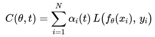
Where:
theta is the set of model parameters.
x_i is the i-th training sample, and y_i is its corresponding label.
f_{theta}(x_i) is the model’s prediction for the i-th sample.
L(...) is the loss function (e.g., cross-entropy, mean squared error).
alpha_i(t) is a time-dependent weight for the i-th sample, indicating how much that sample contributes to the total cost at iteration t.
Under a curriculum-learning approach:
At early training iterations, alpha_i(t) is high for simpler examples and relatively low for complex ones.
As t increases, alpha_i(t) increases for more difficult examples and decreases for simpler ones, placing more emphasis on “harder” parts of the dataset.
Deciding Simplicity vs. Difficulty
One major challenge is to quantify the complexity of an example. Common strategies include:
Using some measure of loss or error for each sample. If a sample consistently produces low loss, it might be considered “easy” and given a lower weight over time.
Pre-calculating difficulty measures based on domain knowledge, such as length of a sentence in natural language processing or presence of certain patterns in images.
Scheduling the Weighting Changes
Designing a good schedule for alpha_i(t) is crucial. A few strategies include:
Linear scheduling: Gradually ramp up the weight for difficult samples in fixed increments.
Adaptive scheduling: Dynamically adjust weights based on real-time metrics (e.g., if the model is performing well on certain classes, the system reduces their weights automatically).
Time-based weighting: alpha_i(t) might be a function of t alone (e.g., some exponential or polynomial decay/growth).
Practical Implementation Concerns
Implementing dynamic cost functions in a modern framework like PyTorch or TensorFlow usually involves:
Maintaining a separate weighting tensor alpha(t) that has one entry per sample or per mini-batch.
Updating alpha(t) at each epoch or iteration based on a chosen rule.
Multiplying the standard loss by alpha(t) before backpropagation.
A possible pseudo-code snippet for PyTorch might look like this:
import torch
import torch.nn as nn
import torch.optim as optim

model = YourModel()
criterion = nn.CrossEntropyLoss(reduction='none')  # 'none' to get loss per sample
optimizer = optim.SGD(model.parameters(), lr=0.01)

def get_dynamic_weights(epoch, difficulty_scores):
    # Implement your logic to generate alpha for each sample
    # For example, simpler samples get weight decayed over time
    alpha = 1.0 / (1.0 + epoch * difficulty_scores)
    return alpha

for epoch in range(num_epochs):
    for batch_x, batch_y, batch_difficulty in train_loader:
        optimizer.zero_grad()
        outputs = model(batch_x)
        per_sample_loss = criterion(outputs, batch_y)

        # Suppose batch_difficulty is precomputed difficulty for each sample
        alpha = get_dynamic_weights(epoch, batch_difficulty)

        # Weighted loss
        weighted_loss = per_sample_loss * alpha
        loss = torch.mean(weighted_loss)

        loss.backward()
        optimizer.step()
Here, batch_difficulty might be a measure of each sample’s complexity (lower means easier, higher means more difficult). Over epochs, the function get_dynamic_weights can shift these alpha values to place heavier emphasis on the harder samples.
Potential Follow-Up Questions
How do you ensure the model is not stuck on easy examples for too long?
One way is to define a precise schedule for transitioning from easier to harder examples. If the model spends too many epochs focusing on easy samples, it might overfit to them. A well-thought-out schedule or an adaptive mechanism for alpha_i(t) helps prevent this. We can also use validation performance as a signal: once validation metrics plateau for simpler subsets, we move to more difficult ones.
What if the easier examples still provide critical gradient signals later in training?
Even if some examples are deemed “easy,” they might still contain valuable information, especially for reinforcing certain model parameters or corner cases. Instead of completely removing easy examples from training, we can give them a small (but non-zero) weight, ensuring the model does not forget previously learned representations.
Could the model overfit on difficult examples once it transitions?
Overfitting is always a concern. One strategy is to apply regularization or keep a small fraction of easier examples at a moderately higher weight to maintain the model’s broader knowledge. Another approach is to cross-validate the weighting schedule to find a sweet spot that encourages learning of complex patterns while not neglecting generalization.
What if we do not have a clear notion of “difficulty” in the data?
In that case, we can estimate difficulty dynamically. For instance, monitor the per-sample loss: if a sample’s loss remains high relative to others, treat it as more difficult. We can also rely on heuristic approaches (like the confidence of the model’s prediction). As the model improves, the relative difficulty can shift, and these shifts directly influence alpha_i(t).
How might you combine curriculum learning with other advanced training techniques?
Curriculum learning can be integrated alongside standard techniques such as:
Data augmentation: Start with mild augmentations (easier) and gradually introduce stronger augmentations (harder).
Transfer learning: Fine-tune a model on simpler tasks or subsets of data, then gradually expose it to more difficult tasks.
Knowledge distillation: Use a teacher model to guide the student model first on simple examples and then ramp up complexity.
Are there real-world use cases where curriculum learning is most effective?
Yes, curriculum learning often shines in scenarios like:
Language learning tasks (e.g., training on shorter, simpler sentences first, then moving to longer, complex structures).
Reinforcement Learning (RL), where initial tasks have simpler reward structures and states, followed by more complex ones as the agent becomes proficient.
Image classification with a wide variance in difficulty, possibly using simpler background or lower resolution images early on and then progressing to more complex scenes.
By thoughtfully designing the dynamic cost function and scheduling how we emphasize examples, curriculum learning can guide a model to learn in a way that mimics human educational processes—starting with the basics and progressively tackling harder challenges once foundational knowledge is established.
Below are additional follow-up questions
How do you measure the effectiveness of a curriculum learning approach during training?
Measuring effectiveness can go beyond just final accuracy or loss. One approach is to keep track of the rate of improvement, especially during different “phases” of the curriculum. For example, you can compare how quickly the model’s performance increases when focusing on easier samples versus how well the model generalizes after incorporating more challenging samples. It is also valuable to monitor metrics that reveal whether the model is robustly learning harder examples. In practice, you can:
Track metrics on subsets of data of varying difficulty. For instance, maintain separate validation sets categorized by difficulty level.
Observe the smoothness of the training curve. An overly steep drop in loss right after introducing harder examples might indicate abrupt changes that could destabilize learning.
Use teacher-forcing or partial inputs for sequences (in NLP tasks) and compare intermediate outputs to see if the model is retaining what it learned from easier stages. A subtle pitfall is overfitting on the easier subset if you spend too many epochs there. So, you want to ensure the shift toward more difficult samples happens at a time when the model stops improving significantly on easy data or begins to show saturation.
When might curriculum learning degrade performance instead of improving it?
One scenario is when the “simpler” examples do not capture the core complexity of the problem, leading the model to learn shortcuts or irrelevant features early on. If these shortcuts conflict with features needed to solve more complex samples, the model may struggle to unlearn them. Another situation is if the transition to harder examples happens too abruptly or too late, causing catastrophic forgetting of previously acquired knowledge or leading the model to be overwhelmed by complexity all at once. A lesser-known edge case arises if your weighting strategy perpetually keeps certain challenging samples at high weights, leading to overfitting on those difficult examples at the expense of overall generalization.
How can we adapt curriculum learning if the data distribution changes over time?
In non-stationary or evolving data scenarios, we may not have a fixed notion of “easy” vs. “hard” examples that remains valid throughout training. Instead, we need an adaptive curriculum that periodically re-evaluates the difficulty of current samples. One approach is to let the model’s own loss determine difficulty on the fly. If the data distribution shifts, certain previously easy examples might become harder for the model and should be reintroduced with higher weights. Another tactic is to incorporate continual learning strategies (like replay buffers or regularization) so that older patterns are not lost. The main pitfall is incorrectly assuming the same difficulty schedule applies to all new data. This can mislead the model if there is a sudden domain shift, so a dynamic re-computation of sample difficulty becomes critical.
How do you handle classes that are consistently more difficult in a multi-class classification task?
In multi-class classification, some classes might naturally present more complexity (e.g., more intra-class variance, fewer training examples, or more confusing boundaries with other classes). One approach is to adjust the curriculum not just at the sample level but also at the class level. You can temporarily increase sampling frequency for these classes if the model is underperforming on them. Additionally, adjusting the loss weights by class can help the model pay extra attention to underrepresented or harder-to-classify classes. A tricky edge case is when certain classes are both difficult and extremely rare. Over-weighting them too early can bias the model too heavily; balancing their representation without overshadowing easier but more frequent classes is often a careful balancing act.
Could we apply dynamic cost weighting in an online or streaming learning context?
Yes, online learning naturally aligns with the ideas of curriculum learning if you interpret “time” as each new batch of streaming data. In an online context, you can maintain a rolling estimate of the difficulty of each data point (for example, by looking at the model’s predicted probabilities or the loss from recent predictions). You can then update the weights for new samples on the fly. A key pitfall is memory constraints: you often cannot keep a large buffer of past samples, so your curriculum might rely on short-term difficulty indicators that can fluctuate significantly. Inconsistent or noisy difficulty measures can lead to oscillations in weighting, making the training process unstable.
How does curriculum learning differ from self-paced learning, and can they be combined?
Curriculum learning is often driven by a predefined notion of difficulty (either determined by domain knowledge or heuristics). Self-paced learning, on the other hand, dynamically selects examples for training based on the model’s current performance (often choosing examples with intermediate loss rather than extremes). Combining them can be beneficial: start with a rough curriculum of easy-to-hard examples, but allow the model to refine which samples to focus on at each stage (self-paced component). The challenge is balancing the two. A pure self-paced approach may neglect certain important but consistently difficult examples if they remain too hard for too long. Meanwhile, a strict curriculum can oversimplify the transition schedule. Merging them carefully requires constant monitoring of how the model interacts with both the predefined curriculum and its own self-assessed difficulty.
How can we avoid catastrophic forgetting when transitioning through different difficulty levels?
One risk in curriculum learning is that once you move on to harder examples, the model may forget what it learned from easier examples. Techniques to mitigate catastrophic forgetting include:
Interleaved training: Gradually sprinkle in some easy examples alongside the harder ones, ensuring they do not vanish entirely from training.
Periodic re-injection of earlier stages: Even if you move the majority of training to complex samples, regularly sample from simpler examples to keep those representations active.
Knowledge distillation: Use snapshots of the model at earlier stages to guide the training of the updated model. This can preserve performance gains from earlier phases. A potential pitfall arises if you re-introduce simpler data too frequently or with too high a weighting, which might slow or undermine progress on more complex aspects.
Could we underrepresent edge cases if we place too much emphasis on an easy-to-hard trajectory?
Some edge cases might be difficult from the outset, but they can also represent critical scenarios in production (e.g., safety-related corner cases in autonomous driving). A strictly easy-to-hard approach can risk deprioritizing or deferring these edge cases for too long. If training ends before these edge cases are thoroughly covered, the model might never learn them well. A balanced curriculum might “mix” a small portion of critical corner cases in even at early phases, ensuring the model is exposed to a broad set of scenarios. One subtle problem is deciding which edge cases are truly important but also not so rare that they distort the entire training procedure.
What overhead does curriculum learning introduce, and how can it be managed at large scale?
Curriculum learning can add complexity in data labeling, difficulty scoring, dynamic sampling, and weight updates. Maintaining a separate weighting factor for each sample could become computationally expensive if you have millions or billions of training instances. Possible solutions include:
Grouping samples into “difficulty bins” to reduce granularity. Instead of weighting each sample individually, you categorize samples into a finite number of bins based on difficulty and assign a single weight per bin.
Updating difficulty levels at epoch boundaries rather than after every iteration, reducing frequency of recalculation.
Using approximate or “lazy” difficulty scoring, where only a subset of samples are re-evaluated for difficulty each time. Pitfalls include losing resolution in difficulty estimation and inadvertently creating new data imbalance if bins are too large or too coarsely defined.
How do you handle incomplete data labels when building a curriculum?
Sometimes in real-world tasks, not all data is fully labeled, or confidence in labels varies. In such cases, you might assign lower priority to samples with uncertain labels early on, to avoid confusing the model with potential noise. As the model matures, it may better handle ambiguous or noisy data. Another strategy is to combine semi-supervised methods (where the model itself generates pseudo-labels) with curriculum principles, letting the model start with high-certainty labeled data and progressively integrate uncertain or partially labeled data. The primary pitfall is that if your labels are incomplete or noisy but also essential for real-world performance, deferring them might hamper the model’s ability to generalize, especially if the domain truly hinges on that uncertain subset.