ML Interview Q Series: When would you remove correlated variables?

📚 Browse the full ML Interview series here.

Comprehensive Explanation

One typical reason for removing correlated variables is to address the problem of multicollinearity. Highly correlated features can create instability in certain models (for example, linear regression). This can lead to inflated variance in the estimated parameters, making it harder to interpret the true relationship between features and the outcome.

There are practical and theoretical motivations for deciding when to remove correlated variables. If a model’s predictive performance is degraded or if coefficients become highly sensitive to small changes in the training data, then removing redundant features is often beneficial. If interpretability is the key goal, dropping correlated variables can help in isolating the effect of each variable on the outcome.

There are also times when you might keep correlated variables. For instance, some algorithms (like decision trees, random forests, or gradient boosting) can better handle correlated variables, since they split the feature space without relying on strict linearity assumptions. In such cases, even if variables are correlated, they might still provide incremental predictive power in subtle, non-linear ways.

Identifying Correlation

A common practice is to calculate a correlation coefficient (for continuous features), or use something like the Cramér’s V statistic (for categorical variables). If the correlation coefficient is larger than a certain threshold (for example, 0.8 or 0.9 in absolute value), it often indicates that two features are conveying largely the same signal. If the model is sensitive to multicollinearity (such as linear or logistic regression), you might remove one of the variables.

When measuring correlation between two continuous variables x and y, one of the central formulas is the Pearson correlation coefficient. It can be expressed as:

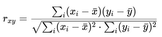
In this expression, x_i and y_i are the individual data points of the respective features x and y. The term x-bar is the mean of feature x, and y-bar is the mean of feature y. The numerator sums the products of the deviations from the mean, while the denominator normalizes by the square root of the sum of squared deviations of each feature, ensuring the result is bounded between -1 and +1. A value close to 1 indicates strong positive linear correlation, a value close to -1 indicates strong negative correlation, and a value near 0 indicates no linear correlation.

Methods to Remove or Reduce Correlation

One direct approach is simply to drop one of the correlated features. A more refined approach is to compute the variance inflation factor (often abbreviated as VIF) in regression settings. A large VIF indicates that the variable is highly explained by other predictors, signaling redundancy. You can systematically remove the variable with the highest VIF, recalculate the VIF for the remaining variables, and continue until all are below a chosen threshold.

Dimension reduction is another popular approach. Techniques like principal component analysis (PCA) effectively transform correlated features into uncorrelated (orthogonal) components that can then be used by your model. This can preserve variance while mitigating the negative impacts of correlation. However, PCA might decrease interpretability because the resulting components are not as straightforward to interpret as the original features.

Code Example for Removing Correlated Variables

import numpy as np
import pandas as pd

# Suppose we have a DataFrame 'df' with numerical features
corr_matrix = df.corr().abs()  # absolute correlation values
upper_triangle = corr_matrix.where(
    np.triu(np.ones(corr_matrix.shape), k=1).astype(bool)
)

threshold = 0.9
to_drop = [
    column for column in upper_triangle.columns
    if any(upper_triangle[column] > threshold)
]
df_reduced = df.drop(to_drop, axis=1)

# 'df_reduced' now has fewer columns and excludes highly correlated variables

This snippet calculates the correlation between all pairs of features, isolates those that exceed a certain threshold, and drops them.

When Exactly to Remove Correlated Variables

One consideration is the final goal of the model. If the model is purely predictive and you are using tree-based algorithms (or other robust methods against correlated features), you might not remove these variables, especially if interpretability is not paramount. In contrast, if you need a regression model with stable coefficients and the ability to interpret each coefficient clearly, then highly correlated variables can cause confounding issues, so it becomes a good idea to remove or merge them.

Another aspect is domain knowledge. Even if two features are correlated, sometimes domain knowledge indicates they capture subtly different phenomena. For instance, if one feature is “number of items purchased online” and another is “time spent on website,” the two might be correlated, but they capture different aspects of user behavior. Some predictive modeling tasks benefit from keeping them both if the algorithm can handle it.

Potential Pitfalls

Overzealous removal of correlated variables might lead to information loss, especially if the correlation threshold is too conservative or if the correlation measure used is not suitable for the feature type. Blindly removing features without domain or data distribution considerations can diminish the signal in your data. Always cross-check the impact on model performance when removing features.

Another subtle pitfall is that correlation is usually measured pairwise. You might remove a feature because it is correlated with one variable but inadvertently lose new or useful information that feature has in combination with other variables. It is sometimes better to use a multi-dimensional approach (like dimension reduction) rather than purely dropping features.

Follow-up Questions

How do you measure correlation among variables of different types?

Correlation in the strict Pearson sense applies to numeric variables with a linear relationship. If one or both variables are categorical, you could use other correlation measures such as Spearman’s rank correlation (for ordinal data) or Cramér’s V for nominal data. In practice, you should choose a measure that captures the relationship type. If it is a monotonic relationship, Spearman’s rank might be more relevant than Pearson’s. If both variables are purely nominal, Cramér’s V measures association without implying linearity.

When might you decide to keep correlated variables?

In decision trees, random forests, and gradient boosting methods, correlated variables can sometimes be complementary rather than merely redundant. If interpretability is not a core objective, you might keep correlated variables to maximize predictive power. In neural networks, correlated inputs can still help the model learn complex representations, especially if each correlated variable captures slightly different nuances of the data. Empirical testing (via cross-validation) often guides the final decision.

How does dimensionality reduction like PCA compare with just removing correlated features?

Removing correlated features is a more direct approach that retains interpretability of the remaining original features. PCA transforms features into linear combinations (principal components). These components are orthogonal by design, thus removing linear correlations, but the downside is that interpretability of each principal component can be more challenging. PCA can preserve most of the variance in fewer features, potentially boosting computational efficiency and avoiding overfitting.

Are there scenarios in which correlated variables are beneficial for interpretability?

Sometimes domain experts want to see certain features in the model even if they are correlated, particularly if those features align with important business metrics or known causal variables. Including them can help discussions with stakeholders, even if purely from a modeling standpoint they are redundant. However, this can be a trade-off, because high correlation can diminish confidence in the coefficients’ significance for each correlated feature.

How does correlation affect regularization techniques such as Ridge or Lasso?

Ridge regression mitigates the effect of correlated variables by shrinking their coefficients, potentially allowing correlated variables to remain in the model but at smaller magnitudes. Lasso regression might shrink some coefficients to zero, effectively removing them. If you have correlated variables in a Lasso setting, the algorithm might pick only one variable from that correlated set and assign the rest zero. This can be beneficial if you want feature selection, but it can also be somewhat arbitrary if multiple correlated features are equally informative.

Below are additional follow-up questions

How do you handle correlated categorical variables?

When dealing with categorical variables, correlation can manifest in a different way compared to numeric features. Instead of using Pearson correlation, you might investigate correlation through contingency tables or metrics such as Cramér’s V for nominal data. If two categorical features exhibit high association (for instance, they almost always occur together), retaining both may not add much extra information. In practice, you can merge categories, drop one variable, or consider more advanced feature engineering approaches.

A subtle pitfall is that a low cardinality categorical feature (a feature with only a few possible levels) might still bring value if one of its levels is predictive in certain conditions. Even if there is a strong overlap with another feature, the unique level-specific information might be lost if you remove it. Another subtlety arises if the categories partially overlap but are not identical. For instance, “color of product” might be correlated with “season of purchase” if customers tend to choose bright colors in summer. Although correlated, each might still improve the model in certain subgroups of users.

What is the difference between correlation and causation in this context?

Correlation indicates that two variables move together in a pattern—when one changes, the other tends to change in a related way. Causation requires that changes in one variable directly produce changes in the other. In the context of removing correlated features, it is critical to remember that correlation does not necessarily imply a causal connection.

One danger is discarding a variable that is actually the true cause of changes in the target, while retaining a correlated but less meaningful variable. Conversely, if your goal is solely predictive performance, you might not be as concerned about causal relationships. Still, removing the truly causal variable could degrade interpretability. Hence, domain knowledge becomes vital for deciding which of the correlated features is more meaningful to keep.

How do you handle partial or conditional correlation when deciding to remove features?

Partial correlation measures the relationship between two variables while controlling for the effect of one or more additional variables. Conditional correlation generalizes that idea. Sometimes, you might find that two variables seem correlated initially, but after accounting for another key predictor, that relationship is diminished or disappears.

This suggests a more nuanced approach to feature selection: a simple correlation matrix might be too superficial. If your problem requires deeper insight into how variables interact, you can investigate partial correlation networks or advanced statistical procedures such as structural equation modeling. However, these methods can become quite involved. A pitfall is that partial correlation analyses may require strong assumptions about the relationships among variables. If those assumptions are violated or if the sample size is small, the partial correlation estimates can be misleading.

How do you handle correlated variables when the correlation structure changes over time, as in time series data?

In a time series context, correlations between variables can be non-stationary, meaning they shift over time. What was correlated in one time window might become less correlated in another. If you rely on a static correlation threshold based on historical data, you risk making suboptimal decisions when the underlying relationships evolve.

One way to handle this is by using rolling or expanding windows to estimate correlations dynamically. You observe how the correlation changes over time and adapt your feature selection accordingly. However, you should be careful: if you frequently drop and add features, your model might become unstable in production. A practical approach is to set a robust threshold for correlation that has been tested across multiple time windows, and only remove features if they remain consistently above the threshold over a prolonged period.

What if multiple variables are correlated with each other but not perfectly? Do you remove all, some, or none?

In realistic datasets, it is common for several features to be moderately correlated without any pair exceeding a standard threshold (like 0.8 or 0.9). If you see a cluster of variables that are moderately correlated, one approach is to use dimensionality reduction techniques (like PCA) to capture most of their joint variance in fewer components. This retains much of the information while mitigating collinearity concerns.

Another approach is to use regularization methods (like Ridge or Lasso) to let the model choose how much to weight each variable. If you use Lasso, some of these moderately correlated features might end up with zero coefficients. Alternatively, you can selectively remove the feature that adds the least to predictive power, judged by cross-validation. A pitfall of removing features in a stepwise approach is that you might remove a variable that is less predictive on its own, but in combination with others could have provided additional predictive signal.

How does correlated variables affect logistic regression models specifically, especially with interpretation of odds ratios?

In logistic regression, each coefficient corresponds to the log-odds change of the target variable given a one-unit change in the predictor while holding all other variables constant. If two variables x1 and x2 are highly correlated, it is difficult to hold x1 constant while changing x2, because in practice, x2 tends to change alongside x1.

As a result, the coefficient estimates can become unstable, and the odds ratios might be misleading. In extreme cases, the maximum likelihood estimation can fail to converge if multicollinearity is severe. If interpretability is essential, you may remove or combine correlated features so that the coefficient estimates more reliably reflect individual effects.

Are there scenarios in which you might transform correlated features instead of removing them?

Sometimes applying transformations—like taking ratios, differences, or other combinations—can convert correlated variables into a single more interpretable and less redundant feature. For instance, if “salary” and “expenditure” are highly correlated, you might consider “savings = salary - expenditure” or a ratio “expenditure/salary” to capture the proportion of income spent.

A subtlety is that such transformations presume a specific relationship. If you incorrectly transform variables, you might lose important nuances or introduce unnatural relationships. A common pitfall is to create transformations that overfit the training data or do not generalize. It is wise to validate whether the transformed feature outperforms or maintains comparable performance relative to the original features.

How does correlated variables influence automated feature selection methods, like forward selection or backward elimination?

In forward selection, features are added one by one based on some criterion (often improvement in an evaluation metric). If two features are highly correlated, adding the second feature might show only a small incremental gain, which could cause it to be skipped. Conversely, backward elimination starts with all features and removes them one at a time. If two features are correlated, whichever is deemed “less critical” might be removed first, even if the difference in importance is small.

One edge case arises when a feature set includes a variable that is individually important but is overshadowed by a correlated variable that was selected first. This may prevent an otherwise useful feature from being added (in forward selection) or retained (in backward elimination). Consequently, these stepwise methods can be suboptimal unless carefully monitored. Cross-validation performance and domain knowledge should guide whether correlated features are genuinely redundant or might add incremental value.

How do you systematically pick a correlation threshold, and might the threshold differ depending on the model or domain?

Choosing a cutoff for “high correlation” (for example, 0.8 or 0.9) is somewhat subjective and context-dependent. A threshold that is appropriate in a medical study (where interpretability and minimal redundancy might be crucial) might be too strict or too lenient in a marketing application. One practical approach is:

1. Consider the statistical properties of the data: if variables tend to cluster around 0.6–0.7 correlation, setting a threshold of 0.7 might remove a large fraction of variables.

2. Conduct a sensitivity analysis: remove correlated features at different thresholds and see how model performance and interpretability change.

3. Factor in model type: for linear regression or logistic regression, even moderate correlations can be problematic. For tree-based methods, you might be more lenient.

A subtle pitfall is to rely solely on a correlation matrix for deciding the threshold. Some features might become correlated only in certain subgroups or under certain conditions. A thorough analysis includes looking at partial plots, domain knowledge, and performance metrics.

Could correlated variables signal data leakage or unintentional redundancy in the dataset?

High correlation might sometimes reveal data leakage. For instance, if two features are supposed to measure different aspects of a problem but are suspiciously identical or nearly identical, it might indicate that one feature effectively “encodes” the label or a post-outcome measurement. This would artificially inflate performance in training but fail in real-world scenarios. Investigating the reason behind suspiciously high correlations can reveal overlooked data leakage, duplicates, or measurement errors.

A subtle challenge is that data leakage might not be obvious if the correlation is strong but not perfect. For example, a variable capturing user behavior after an event that is correlated with the user’s eventual conversion might still be partially leakage. Always scrutinize how each feature is created and ensure that it is available at prediction time without using future or outcome-derived information.