ML Interview Q Series: When would you remove Correlated Variables?

📚 Browse the full ML Interview series here.

Comprehensive Explanation

Correlated variables often carry redundant information. In some machine learning models, especially those that assume independent predictors (like linear or logistic regression), having highly correlated features (multicollinearity) can cause instability in parameter estimates and affect interpretability. This is because when variables are highly correlated, the model may struggle to discern their individual effects on the target. However, whether or not you remove correlated variables can depend on the type of model and your overall goals:

In linear models, strong correlations among features can inflate variance of coefficients and make them unstable. This makes it difficult to interpret which predictor is driving changes in the output. Sometimes, removing correlated variables helps ensure the remaining features contribute unique information to the model.

In tree-based models (e.g., Random Forest, Gradient Boosted Trees), correlated features are less problematic from a performance perspective because these models can pick whichever feature is more important at each split. However, interpretability might still suffer if many variables convey overlapping information.

In high-dimensional problems, correlated variables can cause increased computational load and can complicate the learning process. Reducing them can help avoid overfitting and shorten training times.

Below is the mathematical expression for Pearson’s correlation coefficient, which is a common way to measure linear correlation between two continuous variables x and y.

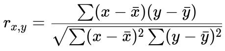
Here, x and y are the observed values for two variables; x̄ (x-bar) and ȳ (y-bar) represent their respective means. The numerator is the covariance term, and the denominator is the product of the standard deviations of x and y. The value of r ranges from -1 to +1, where -1 indicates a perfect negative linear correlation, +1 indicates a perfect positive linear correlation, and 0 means no linear correlation.

Model types that rely on an assumption of independence or have high sensitivity to feature scaling typically suffer more from high correlation among input variables. Hence, in those scenarios, you might remove or combine correlated variables (e.g., by taking the average, principal components, or other dimensionality reduction approaches).

How to Decide When to Remove Correlated Variables

You might decide to remove correlated features to reduce model complexity or to make your model more interpretable. If two variables are nearly duplicates (like weight in kilograms vs. weight in pounds), you gain little by keeping both. Also, in scenarios like stepwise linear regression for interpretability, removing correlated variables can help produce more stable coefficient estimates.

In practice, it’s common to compute the correlation matrix before modeling, identify pairs of features whose correlation exceeds a threshold (like 0.8 or 0.9), and remove or transform some of them. The choice depends on your domain knowledge as well; if you know one variable is easier to measure or more relevant, you can drop the other.

Why Models with Penalties Might Still Keep Correlated Variables

Some linear models (like Lasso or Ridge regression) can handle correlated predictors without requiring you to explicitly remove them beforehand. Ridge regression (L2 penalty) shrinks the coefficients of correlated variables towards each other, while Lasso (L1 penalty) often pushes coefficients of lesser-important variables to zero, effectively performing feature selection. Even so, in extreme cases of multicollinearity, removing highly correlated variables can make the model more stable and simpler.

Example Code to Identify and Remove Correlated Variables

import pandas as pd
import numpy as np

# Example dataset
data = {
    'A': [1, 2, 3, 4, 5],
    'B': [2, 4, 6, 8, 10],  # B is highly correlated with A
    'C': [1, 1, 2, 2, 3]
}

df = pd.DataFrame(data)

# Calculate the correlation matrix
corr_matrix = df.corr()

# Set a threshold for correlation
threshold = 0.8

# Find the pairs of features that have correlation above the threshold
to_remove = set()
for i in range(len(corr_matrix.columns)):
    for j in range(i + 1, len(corr_matrix.columns)):
        if abs(corr_matrix.iloc[i, j]) > threshold:
            colname_j = corr_matrix.columns[j]
            to_remove.add(colname_j)

df_reduced = df.drop(columns=to_remove)
print("Original columns:", df.columns)
print("Columns removed:", to_remove)
print("Remaining columns:", df_reduced.columns)

In this example, you can see how to compute the correlation matrix, identify variables whose absolute correlation is greater than some threshold, and remove them from your dataset.

Follow-up Questions

What if the Model is Tree-Based? Should Correlated Variables be Removed?

Tree-based methods can handle correlated features relatively well. They effectively choose splits across variables and can end up using the most predictive features first. However, if you want a smaller feature set or aim to interpret feature importance, it might still be reasonable to remove redundant features. Correlated variables can mask each other’s importance, making it harder to explain how the model makes predictions.

How Do We Handle Categorical Correlations?

Categorical features can also be correlated, though we often discuss “association” rather than linear correlation. One approach is to use methods like the chi-square test or Cramer’s V statistic to measure associations in categorical variables. If you discover strong associations among categorical features, you can similarly choose to remove or combine them. The principle of removing redundant features remains the same, but you use appropriate statistical measures for categorical data.

Are There Cases Where We Might Keep Highly Correlated Features?

Yes. If your aim is purely predictive and you’re using a model robust to multicollinearity (such as tree-based models or penalized linear models), you might retain correlated features to ensure maximum predictive signal. Another scenario is if the correlated variables each have separate, meaningful domain interpretations. In domains like medicine, each variable might be important to domain experts despite correlations, so they might prefer to keep them for interpretability or domain-specific insights.

Do Correlated Variables Impact Dimensionality Reduction Methods Like PCA?

Yes. Principal Component Analysis (PCA) is based on capturing directions of maximum variance in the feature space. If your features are strongly correlated, PCA will compress that correlated variation into fewer principal components, often reducing dimension effectively. You may not have to remove correlated variables manually in such cases, because PCA or other decomposition methods will automatically project correlated features into lower-dimensional subspaces. However, interpretability might become more challenging, since the new components are linear combinations of your original variables.

Below are additional follow-up questions

What if the Correlation Between Features Changes Over Time? How Do We Handle That?

Correlation is not always static. In many real-world scenarios (e.g., financial time series, streaming data from IoT sensors), the relationship between features might shift due to changes in external conditions or system dynamics. If we train on historical data and the correlation structure changes in the future, the model may perform poorly.

One approach is to perform rolling or sliding-window correlation checks. Rather than compute correlation once on the entire dataset, you compute correlations at different time intervals and observe how they evolve. If you see that certain variables become highly correlated only during specific periods (e.g., seasonal changes), you can decide whether to drop them or transform them in a way that accounts for the shifting relationship.

Edge cases and pitfalls:

You might remove features prematurely if the correlation is temporary or noise-driven. If you have limited data or if a system experiences abrupt regime shifts, a rolling-window correlation check might not capture changes rapidly enough. You should be sure that changes in correlation are not solely the result of a small number of outliers.

What If There Is a Nonlinear Relationship Rather Than a Linear Correlation?

Traditional correlation metrics like Pearson’s correlation coefficient capture linear relationships. Two variables could have a strong nonlinear relationship but appear to have near-zero linear correlation. In such a situation, dropping variables based on linear correlation alone could be misguided.

Alternatives include methods like Spearman’s rank correlation (which measures monotonic relationships) or mutual information (which can capture more general dependencies). For many real-world datasets, nonlinear relationships are common (e.g., quadratic, exponential, sinusoidal).

Edge cases and pitfalls:

A variable pair might not show a linear correlation but still has a significant impact on the model through nonlinear interactions. Using rank-based or mutual-information-based methods requires more computational effort and might be sensitive to how you bin or rank data. Even with a strong nonlinear association, the best approach might be to engineer features that represent that relationship, rather than dropping or keeping both variables without further transformation.

How Do We Handle Partial Correlation?

Partial correlation measures the degree of association between two variables while controlling for the effect of one or more additional variables. This can be useful when you suspect that two variables appear correlated because of a third (or multiple) confounding variable(s).

Below is the formula for a partial correlation between variables x and y while controlling for a variable z (all are continuous):

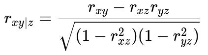
Here, r_{xy} is the correlation between x and y, r_{xz} is the correlation between x and z, and r_{yz} is the correlation between y and z. If r_{xy|z} is small but r_{xy} is large, it suggests that x and y were primarily correlated because of z.

Edge cases and pitfalls:

Partial correlation requires you to specify which confounders to control for, and that depends on domain knowledge and data availability. With high-dimensional data, computing partial correlations can be computationally heavy. Multicollinearity among the confounding variables themselves can affect the stability of the partial correlation estimates.

How Do We Handle Correlation in Neural Networks?

Neural networks often learn complex patterns, including potential redundancy among input features. In principle, a sufficiently large network can learn to disregard redundant inputs if they don’t contribute to minimizing the loss. However, correlated variables can still cause:

Longer training times, as multiple redundant signals might complicate the gradient landscape. Reduced interpretability, because weights associated with correlated inputs can be spread out or duplicated across neurons, making it difficult to know which input is truly driving decisions.

Practical considerations include performing a correlation check before training to remove features that are obviously redundant. Alternatively, dimensionality reduction methods or autoencoders can help discover latent factors that compress correlated inputs into more meaningful representations.

Edge cases and pitfalls:

In extremely large neural networks (e.g., deep architectures with huge capacity), the network might still learn from correlated features without significant performance degradation, so you might not see a large negative effect. Correlated features might cause unstable training if your batch sizes are small or your initialization scheme interacts poorly with the correlated inputs.

Do We Need to Re-check Correlations After Data Transformations?

Many feature engineering steps (e.g., log transformations, standardization, polynomial expansions, encoding) can alter relationships among variables. For example, if you log-transform a heavily skewed feature, its correlation with other features might change significantly.

In practice, it’s a good idea to compute correlations after you perform major transformations or feature engineering. That way, you ensure that you’re making decisions (e.g., removing variables) based on the data’s final representation.

Edge cases and pitfalls:

Repeated transformations (e.g., multiple polynomial expansions) can inadvertently inflate dimensionality and create new correlated features. If you use non-linear transformations, the correlation might become more or less apparent, and relying on a single correlation measure (like Pearson’s) might miss these nuances. Always consider the domain context—some transformations are standard practice in certain fields (like log-scaling in finance or biology).

How Do Outliers Affect Correlation and the Decision to Remove Variables?

Outliers can inflate or deflate correlation values. A single extreme point can make two features seem highly correlated (or uncorrelated) even if that relationship is not representative of the majority of the data.

Robust correlation measures (e.g., Spearman’s rank or Kendall’s tau) are sometimes used to mitigate the effects of outliers. If you see that a correlation is driven mostly by a handful of extreme points, you might investigate whether those outliers are valid data points or errors. In some cases, removing or winsorizing outliers stabilizes the correlation measure.

Edge cases and pitfalls:

If your domain naturally produces outliers (e.g., extreme but valid stock market fluctuations), removing them might throw away crucial information. Winsorizing or trimming outliers can help linear models but might distort interpretability for tree-based or neural models. Always investigate the reason behind outliers before deciding how to handle them.

How Does High Dimensionality Complicate Decisions About Correlated Features?

In very high-dimensional scenarios (thousands or millions of features), many pairs of variables could be correlated purely by chance. Methods like dimensionality reduction (PCA, autoencoders) or regularization-based models (Ridge, Lasso) can help systematically reduce feature space. When dealing with extremely large feature sets:

Set a robust threshold for correlation, because with many features even moderate correlations can be statistically significant. Consider advanced feature selection methods that account for correlation in a more global way, such as hierarchical clustering on the correlation matrix, so you can identify clusters of correlated features and pick a representative from each cluster.

Edge cases and pitfalls:

Computational cost of computing a full correlation matrix can be prohibitive (O(n_features^2)), requiring distributed or approximate methods. For streaming or online learning contexts, continuously updating the correlation matrix might be unrealistic. Incremental or sketch-based methods for large-scale data become necessary.

Are There Domain-Driven Reasons to Keep Correlated Features?

In many regulated or specialized domains like healthcare, insurance, or finance, certain features need to remain in the model for compliance or interpretability reasons. Even if they are correlated, their presence might be mandatory to fulfill regulatory requirements or to provide transparency to stakeholders.

For example, a credit risk model might have multiple correlated measures of a borrower’s creditworthiness (e.g., credit score from different agencies). Dropping one might reduce interpretability or stakeholder trust, even if it’s statistically redundant.

Edge cases and pitfalls:

Legal or regulatory frameworks might require the inclusion or disclosure of certain variables. Removing variables without domain consultation can lead to loss of critical signals, or worse, it may violate the rules for building or auditing a model. Sometimes an external entity validates each variable’s presence. Unilateral removal of correlated features could cause compliance issues or the need for re-approval.