
ML Interview Q Series: Which clustering methods are ineffective for datasets with both continuous and categorical features, and why?

📚 Browse the full ML Interview series here.
Comprehensive Explanation
Traditional clustering algorithms like K-means and Gaussian Mixture Models rely heavily on Euclidean distances or continuous probability density assumptions. When dealing with mixed data (continuous + categorical), these methods can struggle to handle the non-numeric or non-ordinal characteristics of categorical variables. Below is a deep dive into why certain algorithms fail in these scenarios and which alternatives you can employ.
Why K-means and Similar Approaches Are Not Suitable
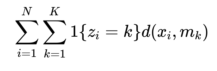
K-means Objective
K-means computes cluster centroids by minimizing the sum of squared distances between each data point and the assigned cluster centroid. The objective function for K-means can be represented in mathematical terms as follows:

Here, i indexes each data point, k indexes each cluster, z_i is the cluster assignment for data point i, x_i is the data point (often in R^d for continuous variables), mu_k is the centroid of cluster k, N is the number of data points, and K is the number of clusters.
Euclidean Distance Assumption: Euclidean distance is a valid measure for continuous numerical data, but it is not naturally applicable to categorical variables. Converting categories to arbitrary numbers or using one-hot encoding can distort distance measurements or introduce high-dimensional sparse vectors that degrade performance.
Centroid Calculation: The mean of categorical values does not have a meaningful interpretation (e.g., the “average” of categories like red, green, and blue is nonsensical). K-means requires a centroid that minimizes variance, but this concept does not directly translate to categorical data.
Gaussian Mixture Models (GMM)
Probabilistic Assumptions: GMM assumes data is generated from a mixture of Gaussians (continuous distributions). Fitting Gaussian parameters to categorical data is not generally meaningful.
Likelihood Computation: For categorical data, the probability density function of a Gaussian is not defined in a way that handles discrete attributes.
In essence, any clustering algorithm that relies purely on continuous distance metrics (like Euclidean) or continuous distributions (like Gaussians) typically is ill-suited for mixed data without special preprocessing or custom modifications.
Algorithms Better Suited for Mixed Data
K-modes for Categorical Data
Instead of means, K-modes computes modes (the most frequent category within each cluster) and uses a simple dissimilarity measure (count of category mismatches) for updating cluster assignments. The objective is often expressed as follows:
Where:
i indexes the data points,
k indexes the clusters,
x_i is the i-th data point,
m_k is the mode (i.e., the most frequent category) that represents cluster k,
d(x_i, m_k) is the number of mismatched categories between x_i and m_k.
This approach is built for purely categorical data, as it uses “mode” updates and categorical mismatch counts instead of variance-based updates.
K-prototypes for Mixed Data
K-prototypes is a hybrid of K-means and K-modes, specifically designed for mixed data:
Continuous Attributes: Uses Euclidean distance, similar to K-means.
Categorical Attributes: Uses the simple matching approach, similar to K-modes.
Combined Cost Function: Balances the contribution of continuous distance and categorical mismatch. You can introduce a weighting parameter that controls how much emphasis to place on continuous vs. categorical dissimilarity.
This method updates “prototypes” rather than centroids, where each prototype contains numeric means for continuous features and modes for categorical features.
Hierarchical Clustering with Gower Distance
For more flexibility, you can use Hierarchical Clustering alongside a distance metric that can handle mixed data types, such as Gower distance. Gower distance splits the similarity calculation for each feature based on its type (numeric or categorical) and then aggregates these similarities into an overall distance.
A simplified representation of the overall Gower similarity between two points i and j can be written as:
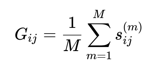
Where:
M is the total number of features,
s_{ij}^{(m)} is the partial similarity between points i and j on feature m. For a numeric feature, it might be 1 - (|x_i - x_j| / range), while for a categorical feature, it might be 1 if the categories match or 0 otherwise.
G_{ij} is then converted to a distance metric by taking (1 - G_{ij}).
Since hierarchical clustering lets you define your own distance matrix, you can easily incorporate Gower distances to handle both numerical and categorical features effectively.
Other Alternatives
Model-Based Clustering for Mixed Data: Some advanced model-based methods can handle discrete and continuous variables by mixing distributions (e.g., using a multinomial for categorical and Gaussian for continuous).
Density-Based Methods with Mixed Metrics: If you can define a valid distance or similarity measure for your data, some density-based algorithms (like DBSCAN) could be adapted, but they still rely heavily on how well that measure behaves in high/mixed dimensions.
Potential Follow-up Questions
How would you handle scaling for continuous features when using K-prototypes?
When continuous features vary in their dynamic range, high-range features can dominate the Euclidean distance compared to lower-range features or categorical mismatch counts. One standard practice is to standardize or normalize continuous attributes (e.g., transform them so that each feature has zero mean and unit variance). This step ensures that no single continuous feature disproportionately affects cluster formation. Additionally, the weighting parameter in K-prototypes can be tuned to balance the influence of continuous distance vs. categorical mismatches.
Is it ever acceptable to encode categorical variables numerically for algorithms like K-means?
It depends on the nature of the categorical variables and their cardinalities:
Ordinal Variables: If there is a natural ordering (small < medium < large), numerical encoding might be acceptable because the variable genuinely has a continuum.
Nominal Variables: If the categories have no intrinsic order (e.g., colors, product categories), direct numeric encoding can artificially introduce ordinal relationships. This can distort cluster formation.
One-Hot Encoding: While common, it often causes issues with K-means due to high-dimensional sparse vectors. Also, Euclidean distance in that space might not accurately represent “similarity” for nominal variables.
In general, specialized methods like K-modes, K-prototypes, or Gower distance are preferred.
Can hierarchical clustering still be used if the data is very large?
Hierarchical clustering can become computationally expensive (often O(N^2) distance computations and memory) as the dataset grows. For large datasets, you might:
Use approximate methods or specialized libraries that employ efficient data structures.
Sample the data and perform hierarchical clustering on a representative subset.
Switch to more scalable algorithms like K-prototypes that typically only require O(TNK) operations per iteration (where T is the number of iterations, N is data size, and K is the number of clusters).
How do K-prototypes and K-modes initialize their modes or prototypes?
Similar to K-means, random initialization is common. However, to improve stability and reduce dependence on random seeds, specialized initialization heuristics are sometimes used:
K-modes: Select random points as initial modes or use a frequency-based approach to choose the most frequent categorical combinations as initial modes.
K-prototypes: For continuous features, it might randomly pick data points or compute the mean of randomly chosen subsets. For categorical features, it might pick the mode from randomly chosen points. Additionally, iterative initialization approaches (similar to K-means++ for numeric data) can be adapted.
Show an Example of Implementing K-prototypes in Python
Below is a simplistic code example using the kmodes package, which supports K-modes and K-prototypes. Note that you would first install the library via pip install kmodes.
from kmodes.kprototypes import KPrototypes
import numpy as np

# Suppose we have a dataset with both numeric and categorical columns
# numeric_cols = [0, 1]  # columns with continuous data
# categorical_cols = [2, 3]  # columns with categorical data

# Dummy data: each row is [numeric1, numeric2, categorical1, categorical2]
X = np.array([
    [5.5, 2.3, 'red', 'typeA'],
    [6.2, 1.8, 'blue', 'typeB'],
    [4.8, 3.1, 'red', 'typeA'],
    [6.0, 2.0, 'blue', 'typeC'],
    [5.0, 2.2, 'red', 'typeA'],
    [6.1, 2.5, 'green', 'typeB']
], dtype=object)

kproto = KPrototypes(n_clusters=2, init='Cao', verbose=2, max_iter=20)
clusters = kproto.fit_predict(X, categorical=[2, 3])

print("Cluster assignments:", clusters)
print("Cluster centroids (prototypes):", kproto.cluster_centroids_)
KPrototypes is initialized with the desired number of clusters.
We specify which columns are categorical via the
categoricalparameter.The algorithm then applies different distance metrics to numeric vs. categorical columns, computing combined distances during the clustering process.
How do you choose between K-modes, K-prototypes, and hierarchical clustering with Gower distance?
All Categorical Data: K-modes is often simpler and directly handles the mismatch measure.
Mixed Data: K-prototypes is generally the most straightforward for tabular data that blends continuous and categorical attributes.
Need for a Dendrogram or Additional Flexibility: Hierarchical clustering (with Gower distance) might be useful if you need to explore multiple cluster resolutions or desire a hierarchical structure. However, it may not be as scalable.
Complex Distributions: If data distribution is more complex, or if some variables are ordinal or count-based, you may consider advanced model-based approaches or carefully designed distance metrics.
What if some features are binary and others are continuous?
Binary features can be considered a special case of categorical variables (with two categories). Any approach capable of handling general categorical variables (like K-prototypes or Gower distance) will accommodate binary features. You just need to be sure to label them as categorical or treat them with a 0/1 mismatch approach if using something like K-modes or K-prototypes.
Could you use a density-based method like DBSCAN for mixed data?
DBSCAN can be adapted if you provide a custom distance function that properly handles mixed data (e.g., Gower distance). However:
Parameter Sensitivity: DBSCAN relies on parameters such as
eps(neighborhood radius) andmin_samples. With mixed data and custom distances, tuning these parameters can be tricky.Computational Overhead: Computing and storing all pairwise distances (for large datasets) can be expensive.
Interpretability: DBSCAN might yield several small clusters or treat many points as noise if distance thresholds are not chosen carefully.
Thus, while technically feasible, you must ensure the chosen distance measure and parameters reflect meaningful similarity across different data types.
Potential Pitfalls and Edge Cases
High Cardinality Categorical Features: If a dataset contains categorical features with many unique values, the cluster prototypes might not converge easily, and the distance calculations can be less stable.
Imbalanced Feature Scales: When numeric features have different ranges, they can overshadow categorical mismatches or vice versa. Proper scaling and weighting can mitigate this.
Sparse Data: One-hot encoding for categorical variables with many categories can lead to extremely sparse high-dimensional data, which complicates distance-based methods. Consider more direct categorical handling if possible.
Mixed Nominal and Ordinal Data: Some categorical variables might be ordinal (like rating scales), some purely nominal (like color). Make sure your chosen approach or distance metric aligns with each feature’s nature.
Overall, whenever continuous and categorical variables coexist, K-means, GMM, or any purely Euclidean-based method typically falls short. K-prototypes, K-modes, or hierarchical clustering with Gower distance are more appropriate alternatives that respect the distinct nature of different feature types.
Below are additional follow-up questions
What if you have multi-level or highly unbalanced categorical variables—how can you adapt your clustering approach?
When categorical features have many distinct levels (sometimes in the hundreds or thousands), clusters can become fragmented. This can occur because each category might appear in only a handful of data points or might dominate most observations if it is extremely frequent. In such scenarios:
Dimensionality Reduction: Consider grouping rare categories together into an “Other” category or using domain knowledge to merge logically similar categories.
Frequency-Based Encoding: Instead of direct one-hot encoding, you might encode categories by their frequencies or weight them by how rare or common they are within the dataset.
Impact on K-prototypes: If the categorical feature has a very large cardinality, the mismatch measure might not be meaningful for categories with extremely small counts. Ensuring the weighting factor in K-prototypes is tuned to address this imbalance is crucial.
Edge Cases: If a rare category appears only once, it can form a tiny singleton cluster if the clustering algorithm heavily penalizes mismatches. This might be undesirable or might reveal a meaningful outlier, depending on your domain context.
How do you handle missing data, especially when both numeric and categorical variables contain nulls?
Handling missing data in mixed-type clustering can be nontrivial:
Simple Imputation: For numeric features, you might impute with mean or median; for categorical features, you might impute with the mode. However, this can artificially reduce variance or misrepresent category frequency.
Distance-Based Approaches: Methods like hierarchical clustering with Gower distance can skip a feature’s contribution if it’s missing for one or both points, effectively computing partial similarities. But if many features are missing in large proportions, distance computations become less reliable.
Separate Category for Missing: Sometimes, you can treat missing values in a categorical variable as its own category, especially if the fact that data is missing is informative. For numeric data, you might use a separate indicator flag along with an imputed value.
Pitfalls: Over-imputation can distort cluster boundaries, and ignoring missing data might drastically reduce the dataset size. Each approach must be tailored to the domain. For example, in medical data, missing values might not be random and could correlate with disease severity or other factors.
Can we treat ordinal variables differently from purely nominal variables, and does this matter for clustering?
Yes, it can matter significantly:
Ordinal vs. Nominal: Ordinal variables (e.g., “low < medium < high”) carry a sense of order, whereas nominal variables (e.g., “cat,” “dog,” “bird”) have no intrinsic order.
Potential Approaches:
For ordinal variables, some distance metrics can penalize distances based on rank differences (such as using numeric 1, 2, 3 to represent low, medium, high) but only if that numeric assignment truly reflects consistent spacing.
With Gower distance, there’s a specific formula for handling ordinal variables that normalizes by the range of possible ranks. This approach preserves the ordering and relative distance between categories.
Edge Cases: If you mistakenly treat ordinal data as nominal, you lose the ordinal relationships. Conversely, forcing a numeric representation on a nominal variable can introduce artificial distances. The correct choice depends on whether the “gaps” between categories are meaningful.
How do you interpret the results of K-prototypes or K-modes, especially when prototypes comprise both numeric and categorical modes?
Interpreting cluster prototypes requires combining numeric means or medians (depending on your implementation) with the most frequent categorical values:
Numeric Part: A prototype might have a vector of mean values for continuous features. You interpret these as “representative” numeric trait(s) of a cluster.
Categorical Part: The prototype’s categorical mode is the category that appears most frequently in that cluster. This doesn’t capture nuances if multiple categories are common.
Potential Pitfalls:
A single mode doesn’t convey distribution within the cluster. If you have a near-split among categories, the mode might be misleading.
Outliers in continuous features can skew the mean. Median-based prototypes or robust estimates might be better in the presence of extreme values.
Actionable Insights: If your cluster prototype for a particular cluster is
[5.2, 3.8, "blue", "typeB"], that means on average, numeric features center around 5.2 and 3.8, and the most common category among cluster members is “blue” for the first categorical feature and “typeB” for the second. Domain knowledge helps decide if this grouping is logical or if further splitting is needed.
How do you measure the quality of clusters when the data is mixed-type?
Evaluating mixed-type clusters is trickier than purely numeric clusters. Some common strategies:
Silhouette Score with Mixed Distance: You can compute a silhouette score using a combined distance metric (like Gower). This gives you a measure of how well-separated the clusters are.
Internal Indices: Metrics like the Davies–Bouldin or Calinski–Harabasz index can be adapted if your chosen distance measure generalizes to mixed types. However, not all standard metrics translate perfectly to non-Euclidean distances.
External Validation: If you have labels or partial labels, you can compute purity or Rand index to gauge how well your clusters align with known categories.
Qualitative Assessment: Sometimes, domain experts interpret cluster prototypes or sample cluster members to determine if they make sense in context.
Edge Cases: A single cluster that lumps everything together might yield low variance but is meaningless. Too many clusters might trivially separate nearly every point. Balancing interpretability with cluster coherence is key.
How do you handle outliers in numeric features when using a mixed-type clustering method?
Outliers can disproportionately affect numeric distances and cluster assignments:
Winsorization or Capping: You can bound extreme values at a certain percentile (e.g., 1st and 99th percentiles) to reduce the impact of outliers on distance calculations.
Robust Scaling: Instead of min-max scaling or standardization, use robust scalers that rely on median and interquartile ranges. This helps reduce outlier influence.
Specialized Distance Metrics: Gower distance for numeric features typically normalizes by range, so outliers can inflate that range and reduce the relative distance effect. Some variations or parameter tuning might mitigate this.
Separate Treatment: In some scenarios, you might isolate known outliers or handle them with a separate method before clustering. If outliers correspond to rare but important events (like fraud or system failures), you might intentionally keep them separate for a special investigation.
How can clustering be updated incrementally as new data arrives?
In real-world applications, data can be streaming or can change over time:
Online K-prototypes: Similar to how there are online variants of K-means, you can develop an incremental version of K-prototypes. Each new data point updates the current prototype calculations with small adjustments, rather than re-running the entire algorithm from scratch.
Mini-Batch Approaches: Process data in small batches. This helps scalability and can adapt cluster boundaries gradually. Between batches, prototypes or modes are updated similarly to mini-batch K-means.
Challenges:
Ensuring the categorical mode remains representative if categories drift over time or new categories appear.
Dealing with potential cluster “drift” if the distribution changes significantly, which might require re-initialization or merging/splitting of existing clusters.
What if your dataset includes time-series along with categorical and numeric features?
Time-series data adds complexity due to temporal dependencies:
Feature Engineering: Often, time-series are aggregated into summary statistics (mean, trend, seasonality) or shape-based features for each entity, converting them into numeric features that can then be combined with categorical attributes.
Temporal Clustering: If time ordering is crucial, you might use specialized algorithms that account for sequences or use dynamic time warping (DTW) as a distance metric for the numeric portion of time-series. You can still apply K-prototypes or hierarchical clustering if you can define a suitable mixed distance that includes a time-series similarity component.
Edge Cases:
Seasonal or cyclical patterns might be lost if you reduce a time-series to a single numeric dimension (like average).
Sudden changes (e.g., abrupt shifts in behavior) might skew similarity comparisons unless you incorporate those events carefully.
What are some practical strategies if the number of clusters is unknown for K-prototypes or K-modes?
Determining the number of clusters K is often a challenge:
Elbow Method: Adapt the elbow plot concept by plotting the within-cluster dissimilarity (using your mixed distance measure) for different values of K, then look for a “bend” in the plot.
Gap Statistic: Compare within-cluster dispersion to that expected under a null reference distribution for various K. This can be extended to mixed data, though it requires a meaningful approach to generating reference datasets.
Silhouette or Other Internal Indices: Calculate an internal clustering metric (like silhouette width) for different K and choose the one that yields the highest score.
Practical Domain Constraints: Sometimes, business or domain knowledge might limit the feasible number of clusters (e.g., we can’t interpret more than 10 segments in a marketing context).
Edge Cases:
The “true” number of clusters might be large, but the data has many small, tight groups. You could end up with an impractical solution.
Over-clustering vs. under-clustering can both undermine the interpretability and utility of your solution. Balancing domain expertise with statistical indices is key.
How do you handle interpretability when using complex distance metrics like Gower?
While Gower distance is versatile, it can obscure how each feature contributes to the final distance:
Feature-Level Contribution: One approach is to calculate partial distances for each feature. You can then examine how each feature’s distance accumulates to form the final distance between two points. This helps you see which features drive similarity or dissimilarity.
Weighting or Scaling: Gower distance can be modified to weight certain features more than others based on domain importance or reliability.
Visual Aids: If feasible, consider dimension-reduction techniques (e.g., t-SNE or UMAP with a custom distance function) to visualize how clusters separate in 2D. Though you lose direct interpretability in each dimension, you at least see how the data might partition.
Challenges:
Gower distance is less straightforward to interpret than a single Euclidean metric, especially when you have multiple nominal and ordinal variables.
Domain experts may find it unclear why certain points are labeled “close” or “far.” Summaries of partial feature-level distances can aid interpretation but also increase complexity.