
ML Interview Q Series: Which forms of data bias commonly appear in machine learning pipelines, and what are their possible consequences?

📚 Browse the full ML Interview series here.
Comprehensive Explanation
One key concept that arises when discussing biases in data is statistical bias in the estimator. In a statistical sense, bias can be described as the difference between the expected value of an estimator and the true parameter value. This definition can serve as a starting point for understanding how data biases propagate through machine learning models.
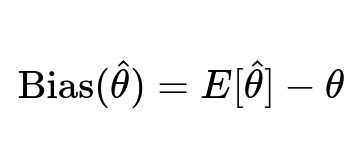
Here, hat(theta) is the estimator (for example, a learned parameter from data), E[hat(theta)] is the expected value of this estimator over different training samples, and theta is the true value of the parameter that we want to estimate. When data are systematically skewed or unrepresentative, the model’s estimator will deviate from the real parameter in predictable ways, resulting in biased outcomes.
Below are common types of biases that can appear in machine learning systems.
Sampling Bias
Sampling bias occurs when the chosen data points are not representative of the overall population. This usually happens if data collection favors certain types of instances. For example, a credit-scoring model trained only on data from people with high incomes will have a distorted view of the population’s creditworthiness. The model might then systematically underestimate or overestimate certain segments of the population.
The main way to mitigate sampling bias is to ensure that sampling procedures are as random and inclusive as possible. In practice, strategies can include stratified sampling (where you proportionally represent each subgroup) or carefully designed data collection methods that cover all relevant sub-populations.
Measurement Bias
Measurement bias arises when the features or labels are measured inaccurately or inconsistently. For instance, if sensors used to gather data for a predictive maintenance model are calibrated differently across different manufacturing plants, the data might reflect those calibration quirks rather than true machine performance. Another form occurs in text labeling, where annotators might systematically misunderstand or misclassify certain categories.
Mitigation often involves standardizing measurement procedures or instrument calibrations, as well as deploying robust labeling guidelines and double-checking how annotations are generated.
Labeling Bias
Labeling bias can be seen when the ground truth labels for training data are themselves flawed or subjective. In many real-world scenarios, labels depend on human judgment. If annotators have preconceived notions—say, about a certain demographic group—this can introduce systematic skew. Over time, the model learns these skewed patterns.
Common remedies include consensus labeling (obtaining labels from multiple annotators and then resolving discrepancies), well-defined annotation guidelines, and thorough training of annotators to reduce subjectivity.
Exclusion Bias
Exclusion bias happens if we intentionally or unintentionally omit important features or data subsets during preprocessing. An example is building a model for student performance but accidentally leaving out features about socioeconomic status. The result is a model that doesn’t account for an influential factor, leading to skewed predictions for different groups.
To address this, thorough feature engineering and domain expertise are crucial. One must carefully investigate whether certain omitted features may inadvertently act as confounders.
Historical Bias
Historical bias is embedded in the data due to past societal or organizational decisions. For instance, if a hiring dataset has historically hired fewer people from certain demographics, the model might continue to favor the majority group. The model inherits the skew from historical patterns, perpetuating biases even if there is no overtly discriminatory feature (like race or gender) in the dataset.
De-biasing methods include re-weighting or re-sampling the data to better reflect the current desired demographics, as well as adjusting decision thresholds to ensure fairer outcomes.
Observer Bias
Observer bias arises if the person or system collecting or labeling data is influenced by subjective expectations. In medical diagnoses, for example, a researcher might consciously or unconsciously record outcomes in a way that fits their hypothesis.
Strategies to reduce observer bias involve double-blind procedures, anonymity in labeling, and standardized data-collection protocols. Moreover, consistent guidelines help ensure that observations are recorded similarly across different observers.
Confirmation Bias
Confirmation bias can occur when data scientists selectively seek or emphasize data that supports an existing hypothesis. In practice, this means ignoring contradictory evidence or failing to test alternative hypotheses. While not limited to data collection, it still affects how datasets are curated and how models are validated.
One safeguard is to implement rigorous data exploration and hold-out validation sets that challenge existing assumptions. Team reviews and peer checks can also make sure no crucial perspectives are overlooked.
Survivorship Bias
Survivorship bias arises when we focus only on entities that “survived” a particular process or event while ignoring those that did not. In predictive modeling, you might end up training only on cases that had successful outcomes, missing all the data from unsuccessful outcomes. This can lead the model to form an overly optimistic picture.
Mitigation typically involves ensuring that data from failed or excluded cases is also captured and analyzed. Properly controlling for these lost samples prevents an overly rosy or skewed analysis.
Reporting Bias
Reporting bias occurs when some findings or data points are more likely to be reported than others, often because of sensationalism, convenience, or cultural norms. For instance, online review data might be disproportionately negative if unhappy customers are far more likely to leave a review. The training data, therefore, paints an unbalanced picture of sentiment.
To handle reporting bias, one might incorporate external data sources or carefully model the likelihood that a particular instance gets reported. Adjusting dataset weights can also help compensate for overrepresented extremes.
Selection Bias
Selection bias arises due to non-random selection of observations into the dataset. This can be thought of as a broader category that includes sampling bias as a subset. Selection bias might happen because the system only records data under certain conditions (for example, only logging data when there is a user interaction, ignoring all other moments).
Mitigation strategies involve thorough auditing of the data collection pipelines, checking for missing segments of the population or time intervals, and possibly weighting instances differently based on how probable they are to be included in the sample.
Practical Tips for Avoiding or Reducing Data Bias
In real-world settings, teams typically combine multiple strategies to reduce bias:
Data Auditing: Regularly examine distributions of key features to detect unusual skews.
Balanced Datasets: Use stratified or balanced sampling to ensure minority groups are not overshadowed.
Feature Engineering: Carefully consider domain-specific features to avoid omitting critical information.
Bias Metrics: Track fairness metrics (e.g., false positive rates for different subgroups) and adjust thresholds or sampling to reduce large disparities.
Human-in-the-Loop Checks: Involving diverse individuals in every stage of data collection, curation, and model evaluation can uncover hidden biases.
What Are Some Real-World Examples of Biased Data?
Biased data manifests in many industries. In healthcare, electronic health records might be incomplete for patients with less frequent visits, causing the model to overlook certain risk factors. In finance, loan approvals might reflect historical biases against lower-income areas. In recommendation systems, user interactions could be biased by popularity, so the system keeps recommending content already widely viewed, perpetuating popularity bias.
What Happens If We Simply Collect More Biased Data?
Collecting more of the same biased data does not necessarily help; it can reinforce existing skew. The root issue is the systematic underrepresentation or misrepresentation of specific groups or features. Merely scaling up the dataset without changing its composition tends to amplify biases, because the model sees even more examples of the same distorted patterns.
Are There Ways to Detect or Quantify Selection Bias?
Several statistical tests can help. One can compare population statistics against the sample’s statistics to see if they match. For instance, if the overall user base is 50% from a particular age range, but your training set has only 5% from that age range, you can quantify the mismatch. In practice:
import pandas as pd

# Suppose df is your dataset, and 'age_range' is a categorical column
overall_distribution = {'18-25': 0.3, '26-40': 0.4, '40+': 0.3}
sample_distribution = df['age_range'].value_counts(normalize=True).to_dict()

# Compare
for k, v in overall_distribution.items():
    print(f"Group {k}: Overall {v}, Sample {sample_distribution.get(k, 0)}")
This kind of simple analysis can give clues on whether certain segments are underrepresented or overrepresented.
How Can We Mitigate Bias in a Large Dataset?
Mitigation can be done at various steps:
Re-sampling or re-weighting to ensure representation.
Correcting or augmenting labels via cross-checks and multiple annotators.
Introducing fairness constraints during training so the model is penalized if it discriminates against certain subgroups.
Regular audits and monitoring post-deployment to detect drift or newly introduced biases over time.
When dealing with large datasets, a system of continuous data auditing is often essential. One should implement automated checks that regularly analyze whether feature distributions and model predictions change significantly over time for each demographic. This approach ensures early detection of any emergent biases.
Below are additional follow-up questions
How do we handle class imbalance as a form of data bias, and what strategies are most effective?
Class imbalance is a specific scenario where one class is significantly more frequent in the training set than others. This is commonly seen in fraud detection, medical diagnostics, and other classification tasks where one “positive” class is rare compared to the “negative” class. The limited examples of the minority class can lead the model to overfit to the majority class and underperform on minority-class predictions.
Strategies to address class imbalance include resampling (oversampling the minority class or undersampling the majority class), generating synthetic data (e.g., SMOTE), using class-weight adjustments in model training, and employing specialized metrics like F1-score, balanced accuracy, or Matthews correlation coefficient instead of raw accuracy. These strategies help ensure that the model does not ignore or underweight the minority class and can improve both fairness and performance.
Potential pitfalls:
Oversampling the minority class can lead to overfitting, especially if the same rare examples are repeated too frequently.
Synthetic data generation can create “borderline” cases that are not truly representative of real-world data, if not carefully tuned.
Class-weight adjustments require parameter tuning. Simply choosing arbitrary weights might solve one form of bias but introduce new forms of distortion in predictions.
Edge cases:
Extreme imbalance cases, such as 1% minority vs. 99% majority, may still be problematic even with advanced techniques. Gathering more real minority data might be the best solution if feasible.
In streaming data, class distributions can shift over time, so online rebalancing strategies or continuous monitoring are needed to keep up with changing class proportions.
Is there a risk that aggressive de-biasing strategies might degrade overall model performance?
When organizations attempt to correct for biases in data, they might apply re-weighting, re-sampling, or other fairness interventions that can shift the model’s underlying data distribution. This shift can alter the global error rate or degrade model performance for the majority group.
From a multi-objective perspective, we may need to balance accuracy and fairness, especially under regulatory or ethical constraints. Some organizations accept slightly lower overall accuracy in exchange for more equitable outcomes among different subgroups. Meanwhile, carefully designed approaches aim to maintain overall performance while reducing bias. Techniques like adversarial de-biasing can be used to preserve relevant predictive power while removing unwanted correlations with protected attributes.
Potential pitfalls:
Over-correction can lead to artificially boosting minority groups, resulting in negative outcomes for the majority group or other non-target subgroups.
Fairness interventions that are not well-calibrated may change the interpretation of predicted probabilities. This can hurt trust in the model if users realize the probabilities no longer reflect real-world likelihood.
Edge cases:
In a highly regulated domain (e.g., lending, hiring), even a minor decrease in overall accuracy might be acceptable if it greatly reduces demographic disparity. In less regulated domains, organizations might place more emphasis on raw predictive performance.
How do biases in feature engineering emerge, and what are the best practices for avoiding them?
Bias in feature engineering can arise when certain features correlate with protected attributes (like age, race, or gender) but are not explicitly recognized as proxies. Including these proxy features can lead a model to learn discriminatory patterns. Also, excluding relevant features out of caution might inadvertently degrade the model’s fairness if the excluded feature could have improved performance for underrepresented groups.
Best practices include:
Conducting thorough correlation analysis to detect strong relationships between features and protected attributes.
Checking for interpretability to see if some features act as unexpected proxies (for instance, ZIP code as a proxy for socioeconomic status).
Applying domain knowledge to decide which features are ethically and legally permissible to include.
Using fairness-driven dimensionality reduction or removing only the components of a feature that are correlated with protected groups.
Potential pitfalls:
Blindly dropping correlated features can harm overall model utility. For instance, removing all location data might degrade the model’s performance in scenarios where geography is highly relevant (like local weather forecasting).
Over-engineering or generating complex interactions can create hidden correlations that are not immediately obvious but can still lead to biased outcomes.
Edge cases:
Highly correlated variables that are essential for predictive tasks. For example, in medical settings, certain demographic factors might be crucial for valid clinical predictions. Striking a balance between fair treatment and clinically necessary correlation is complex.
Could data augmentation or synthetic data introduce new biases?
Data augmentation and synthetic data generation can be used to address underrepresented classes or scenarios. However, the algorithm that generates these new samples has its own assumptions, which might embed new biases. For example, a generative model might fail to capture subtle group differences and produce unrealistic instances.
To mitigate this, practitioners often:
Use high-fidelity generative models that are thoroughly validated.
Conduct domain expert reviews of synthetic samples.
Compare distributions of real vs. synthetic data. If they diverge significantly, the augmentation process might be biased or incomplete.
Potential pitfalls:
Synthetic data might fix the imbalance in numeric terms but fail to capture the diverse characteristics of the minority group. This can still lead to a model underperforming on real minority data.
Augmentation in time-series or sequential data can inadvertently disrupt temporal relationships or correlated features.
Edge cases:
Extreme use of generative data to “invent” entire subpopulations can be ethically questionable and might not reflect any real-world individuals. This may be problematic if the model is then tested on actual individuals with unique traits not well-represented by the generated samples.
How do biases manifest when merging datasets from multiple sources, and how can these be unified fairly?
When combining datasets from different institutions or regions, differences in data-collection methods, definitions of labels, or feature distributions can lead to new biases. For example, one hospital might under-report certain diagnoses compared to another, or one dataset might label certain outcomes differently.
Strategies to unify these datasets fairly include:
Harmonizing feature definitions and data dictionaries across sources. Ensuring that the same feature name corresponds to the same concept.
Applying normalization or calibration techniques to align feature scales and distributions, especially when measurement tools differ.
Conducting thorough exploratory data analysis to uncover any systematic discrepancies between data sources (like differences in patient demographics or testing protocols).
Possibly training models on each dataset separately, then using ensemble methods or meta-learning approaches to reconcile differences.
Potential pitfalls:
Overlooking hidden distinctions (e.g., one dataset uses a broad classification for an outcome while another uses a nuanced multilevel categorization).
Attempting to merge irreconcilable label definitions. For instance, one dataset might define “default on loan” after 60 days of missed payment, while another might define it after 90 days.
Edge cases:
If data from one source is high quality but from another is known to have noisy labels, merging them equally might degrade overall quality. Weighted approaches might help but must be carefully tuned to avoid amplifying bias in the lower-quality portion of the data.
How do we deal with biases that appear or evolve in production after the model is deployed?
Even if a model is carefully trained to reduce bias initially, real-world dynamics can change the data distribution over time—a phenomenon called data drift. New forms of bias can emerge if the user base shifts or if new features influence how data is collected.
To address evolving biases:
Continuously monitor the model’s performance across different segments, looking at metrics like false positive/negative rates or error distributions for each subgroup.
Implement a feedback loop to retrain or fine-tune the model with fresh data that reflects the current environment.
Regularly analyze model outputs to detect unexpected changes in the distribution of predictions across demographic groups.
Potential pitfalls:
Monitoring might be limited to overall accuracy without segment-level breakdown, allowing creeping biases to go unnoticed.
Real-time data might be biased by user behavior or feedback loops (e.g., a recommendation system influencing user interactions, which in turn biases subsequent data).
Edge cases:
In regulated industries, even slight shifts in model behavior can have legal implications if the model appears to systematically disadvantage protected groups. Organizations must be prepared to adjust quickly to remain in compliance.
When might we accept certain biases in the data rather than attempting to correct them?
Some biases reflect genuine, real-world differences that are relevant to model objectives. For instance, an age-related bias in a healthcare model might be valid if older populations genuinely have different clinical risk levels. In such cases, removing the bias could degrade clinical utility.
However, acceptance of biases typically requires:
A clear ethical and domain-specific justification for why the model needs the differentiation.
Transparent communication to stakeholders about the rationale behind including these factors.
An ongoing review to ensure that the bias is indeed medically or domain-relevant, and not a proxy for discrimination.
Potential pitfalls:
Justifying biases without sufficient domain knowledge can lead to accidental discrimination.
Stakeholders might misunderstand the difference between legitimate variance and unfair bias, risking trust in the system.
Edge cases:
Legal or regulatory frameworks might strictly prohibit using certain features (like gender or ethnicity), even if they are predictive in some contexts. One must carefully navigate the distinction between legitimate domain correlation and protected attribute usage.
How can explainable AI techniques help diagnose and mitigate data biases?
Explainable AI (XAI) methods such as SHAP values, LIME, or feature importance plots highlight how each feature contributes to a model’s predictions. By inspecting these explanations, data scientists can see if certain features or data points have an outsized influence on the outcome.
With these insights:
One can spot whether protected or proxy attributes are driving model decisions more than intended.
Stakeholders can hold the model accountable by verifying if its logic aligns with ethical or regulatory standards.
Model debugging becomes more systematic, as suspicious patterns in explanations can guide further data exploration and bias mitigation.
Potential pitfalls:
Explanation methods may provide misleading interpretations if the model is highly complex or if the explanation approach is not well-calibrated.
Over-reliance on local explanation methods can mask global biases if the local explanations appear fair on a small subset of instances.
Edge cases:
Some models are inherently difficult to explain (e.g., large ensembles, deep networks). Implementing XAI might require advanced surrogate modeling or partial dependence analysis, which can themselves introduce approximation errors.
Even if explainability reveals a bias, deciding how to fix it can be non-trivial and requires iterative experimentation.