ML Interview Q Series: Which loss function does k-means minimize, and what are the centroid update formulas for batch and SGD?

📚 Browse the full ML Interview series here.

Comprehensive Explanation

Overview of k-means objective

In k-means clustering, the core goal is to group data points into k distinct clusters, each having a centroid (also referred to as a mean or center). The measure of quality is typically how far points in a cluster are from the centroid of that cluster. The classical formulation of this “clustering quality” is the sum of squared Euclidean distances between each data point and its corresponding cluster centroid.

Squaring the Euclidean distance offers several advantages. It penalizes large deviations more severely and ensures a smooth, differentiable surface that is more amenable to gradient-based optimization techniques.

Why a gradient-based perspective?

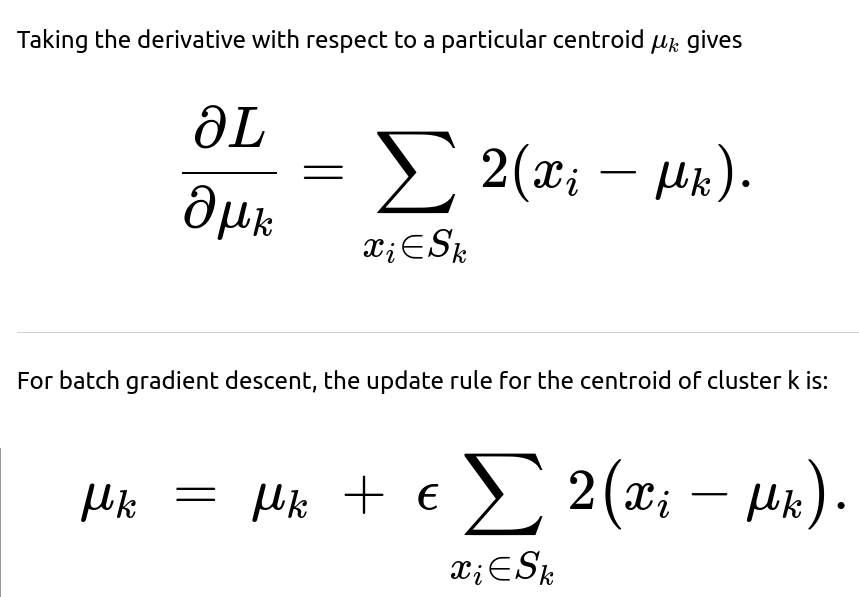
Although the standard k-means algorithm uses an alternating approach of (1) reassigning points to their nearest centroid and (2) recomputing centroids as the mean of assigned points, one can also derive k-means updates from a gradient descent viewpoint. By posing the objective as a sum of squared errors, one can directly compute the gradient of this objective with respect to each centroid and apply update steps. In practice, this leads to the same closed-form mean update if done in batch mode, but can also be extended to streaming or online contexts through stochastic gradient methods.

Mathematical derivation of the objective

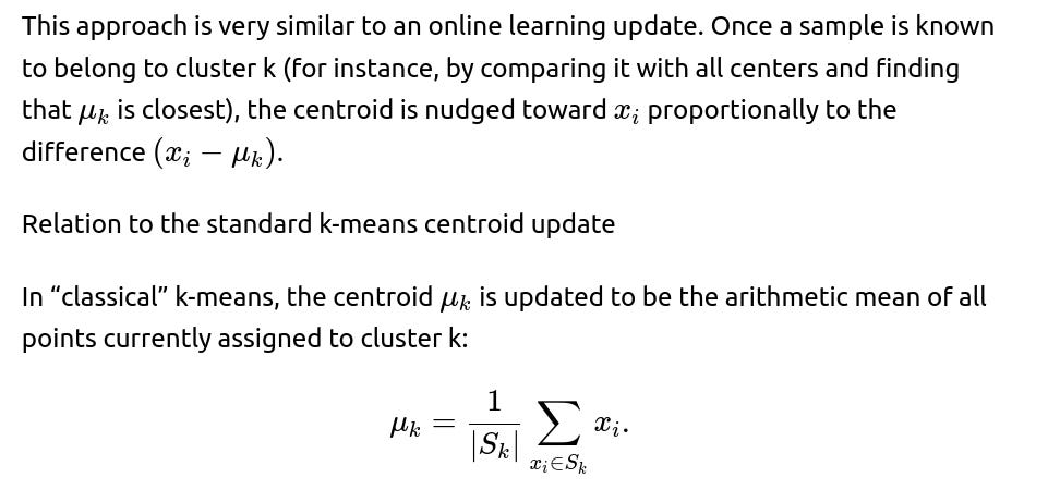
So, the batch gradient descent method, in the limit as the step size goes to a specific value and you take repeated steps, converges to the same result as taking the direct average in one closed-form step. The stochastic update is simply a way of making incremental changes, which is helpful in streaming data or large-scale data scenarios.

Example code snippet (PyTorch style)

import torch

# Suppose we have data points in a PyTorch tensor X,
# and cluster assignments in a list or tensor cluster_assignments.
# cluster_centers is a tensor of shape (k, d).
# We perform a single batch gradient descent step for each cluster.

def batch_update(cluster_centers, X, cluster_assignments, epsilon):
    k = cluster_centers.size(0)
    for cluster_idx in range(k):
        # Gather points belonging to cluster_idx
        indices = (cluster_assignments == cluster_idx).nonzero(as_tuple=True)[0]
        if len(indices) > 0:
            points = X[indices]
            # Compute gradient
            diff = points - cluster_centers[cluster_idx]
            grad = -2.0 * diff.sum(dim=0)
            # Update
            cluster_centers[cluster_idx] = cluster_centers[cluster_idx] - epsilon * grad
    return cluster_centers

def stochastic_update(cluster_centers, x_i, cluster_idx, epsilon):
    # x_i is the single sample assigned to cluster_idx
    diff = x_i - cluster_centers[cluster_idx]
    cluster_centers[cluster_idx] += epsilon * diff
    return cluster_centers

Follow-up question 1

How do we choose an appropriate learning rate for k-means if we are using gradient-based updates?

Follow-up question 2

Why is squared Euclidean distance preferred over other distance measures like the L1 norm in k-means?

The squared Euclidean distance leads to a simple, closed-form solution for the centroid as the mean of the points in the cluster. This is highly convenient computationally. Moreover, squared Euclidean distance is differentiable everywhere, making it more straightforward to apply gradient-based algorithms without dealing with absolute value corners as in L1 norms. While one can define variations such as k-medians (with absolute distances) or k-medoids (with more general distance metrics), these algorithms often become more complex and computationally expensive.

Follow-up question 3

Does k-means always converge to the global minimum of the objective function?

In general, k-means converges to a local optimum rather than a guaranteed global optimum. The loss function has many local minima, and the outcome depends heavily on the initialization of cluster centers. Common techniques to address this include running the algorithm multiple times with different random initializations or using smarter initialization methods such as k-means++.

Follow-up question 4

How can we handle empty clusters during the update process?

Empty clusters can occur if no points are assigned to a particular centroid. This can happen when that centroid is far from all points, especially after certain assignments. Strategies to address empty clusters include:

Re-initializing the empty centroid by randomly selecting a data point or by splitting an existing cluster. Skipping updates that rely on summation over no points. In practice, this means you cannot compute an average. So you must define a fallback rule. Depending on the library or implementation, an empty cluster might be pruned entirely or re-assigned.

Follow-up question 5

What are the main differences between mini-batch gradient descent and standard batch or stochastic approaches in k-means?

Mini-batch gradient descent processes small batches of data points at once, combining some advantages of both batch and stochastic methods. It reduces computational overhead compared to full batch updates (especially on very large datasets), and it typically updates centroids more smoothly than purely stochastic single-point updates. A small batch size can improve efficiency and yield good clustering, though it can introduce a bit of variance in the updates.

Follow-up question 6

Could we use a different distance metric instead of the Euclidean norm?

Yes. While standard k-means is defined with Euclidean distance, variants like k-medians (L1 distance) or k-medoids (arbitrary distance metrics) exist. However, each new metric changes how the centroid is updated. For instance, in k-medians, the best “centroid” is actually the median of the cluster points. For a general metric, there may not be a simple closed-form solution for a centroid, so iterative or specialized methods might be required to find a cluster representative.

Follow-up question 7

How do we typically assign points to clusters in a gradient-based approach?

Though one might think about assigning points via a gradient-based rule, in practice, k-means still uses a straightforward nearest-centroid assignment for each point. Each iteration of a gradient-based approach is effectively refining the centroids. After each refinement step, you can reassign points to whichever centroid is nearest in Euclidean distance. This two-step iterative procedure (sometimes called Expectation-Maximization style steps) continues until convergence.

Follow-up question 8

Does k-means scale well to very large datasets?

K-means in its pure batch form can become computationally expensive for extremely large datasets because each iteration requires scanning all data to compute new centroids. In such scenarios, mini-batch or stochastic updates are preferred. Additionally, algorithms like mini-batch k-means are commonly used in large-scale settings because they allow updates without requiring a complete pass over the entire dataset at each iteration, significantly reducing computational load and memory requirements.

Below are additional follow-up questions

How do we select the number of clusters k in practice?

A common dilemma is deciding how many clusters to create. One popular technique is the “elbow method,” where we compute the clustering objective (sum of squared distances of points to their assigned centroids) for different values of k and look for a point after which further increases in k yield diminishing improvements. Another approach is the “silhouette score,” which measures how similar a point is to its assigned cluster compared to other clusters. Yet another strategy is to use domain knowledge or a known label distribution. Each of these methods can fail if the data does not have well-separated clusters or if there is significant overlap. Moreover, in high dimensions or when the dataset is noisy, the elbow or silhouette methods might not produce a clear-cut optimal k, leading to ambiguity. It is also possible that an organization might have practical constraints (e.g., a marketing campaign might require precisely ten segments).

What are potential issues in high-dimensional spaces for k-means?

In very high-dimensional spaces, distances between points can become less meaningful because of the “curse of dimensionality.” Euclidean distances can concentrate, meaning points can appear almost equidistant from each other. Consequently, k-means may struggle to form coherent clusters. One mitigation strategy is dimensionality reduction, such as PCA, which transforms data into a lower-dimensional subspace that hopefully preserves relevant structure. Another challenge is that any outliers or irrelevant features can dominate the distance computations and distort the clustering. Careful feature engineering, normalization, and sometimes even feature selection can be vital in high-dimensional settings.

How does the presence of severe outliers affect k-means?

K-means uses the mean as the cluster representative, which is sensitive to large outliers because the mean shifts more substantially than, say, the median. In the presence of extreme or numerous outliers, the centroids can be pulled away from the dense regions of normal points. One way to handle this is to use robust clustering variants like k-medoids (which places cluster representatives on actual data points) or trimming outliers as a pre-processing step. Another strategy might involve specifying outlier classes or adjusting the distances with robust metrics. However, trimming outliers can be tricky if the data genuinely contains rare but meaningful instances. Incorrectly removing them can cause important cluster structures to go unrecognized.

How do different initialization strategies affect the final clustering solution?

K-means is sensitive to initial centroid placement. Random initialization may lead to poor local optima or slow convergence. Various initialization schemes exist, with k-means++ being one of the most popular. K-means++ spreads out initial centers by assigning each next center with probability proportional to its distance squared from already chosen centers. This often improves clustering results and speeds up convergence compared to naive random starts. However, even k-means++ can fail in certain pathological data distributions, and multiple runs with different random seeds may still be necessary. Some implementations average results across several runs to mitigate the variability caused by random initialization.

How do we evaluate the quality of clusters when ground truth labels are not available?

In many real-world clustering tasks, there is no label information to measure the “correctness” of clusters in a purely supervised sense. Instead, a variety of internal evaluation measures or unsupervised quality metrics are used. Apart from the within-cluster sum of squares (the k-means objective itself), metrics like the silhouette coefficient or Davies–Bouldin index are popular. Silhouette measures how well each point fits in its cluster compared to other clusters. Davies–Bouldin tries to capture the separation between clusters relative to their internal dispersion. A pitfall is that these metrics might not align with domain-specific notions of a “good cluster,” so domain knowledge often plays a crucial role in validating clustering results.

Is there a risk of centroids getting “stuck” in local maxima when using gradient-based approaches?

When formulating k-means with a gradient method, each update step only looks at the local gradient. Due to the nonconvex nature of the k-means objective, the algorithm can settle into local minima (which in gradient terms might be stationary points of the objective). This is a well-known phenomenon in standard k-means as well. While repeated random restarts can alleviate the problem, there is no general guarantee of finding a global minimum. Practitioners typically do multiple runs and choose the best result based on the objective or other criteria.

Can we accelerate k-means updates with GPU computation or distributed systems?

Yes. Because k-means typically involves repetitive computations of distances between points and centroids, the operations can be vectorized. Libraries such as PyTorch, TensorFlow, or specialized frameworks can leverage GPUs to speed up distance calculations and centroid updates in parallel. For massive datasets spread across multiple machines, distributed k-means algorithms (e.g., using MapReduce, Spark, or other frameworks) are often employed. A subtle challenge in a distributed environment is gathering partial sums or partial centroid updates and then averaging them efficiently. Communication overhead can become a bottleneck, so designing the workflow to reduce network traffic is crucial.

How do we handle mixed data types (e.g., numerical and categorical) in a single k-means approach?

Standard k-means assumes a vector space where distances (Euclidean) make sense for numerical features. If you have a mix of continuous, discrete, or categorical variables, raw Euclidean distance may be inappropriate. One approach is to transform categorical data into a numerical embedding (e.g., one-hot vectors) and then apply standard scaling. However, if there are many categorical levels, one-hot vectors can greatly increase dimensionality and dilute distance meaning. Alternative approaches might involve domain-specific distance metrics or adopting algorithms designed explicitly for mixed data (e.g., k-prototypes, which handles both continuous and categorical attributes). Pitfalls include incorrectly weighting numeric vs. categorical features, leading to clusters that do not meaningfully reflect the domain.

How can convergence be monitored or guaranteed in an online or streaming version of k-means?

In an online or streaming approach (stochastic or mini-batch updates), you continually adjust centroids based on incoming data. Convergence is less clear-cut because new data keeps arriving and updates happen in a streaming fashion. One heuristic is to track changes in centroid positions or the overall objective after each batch. If the centroids shift below a threshold or the objective improvement is negligible, you could declare convergence. However, if the data distribution shifts over time (concept drift), the algorithm might never strictly converge. In that scenario, you might allow the model to adapt indefinitely. A subtle pitfall is deciding when to “stop learning” if your data stream stabilizes, or how aggressively to adapt if the data distribution changes quickly.

Is it possible to allow partial or fuzzy membership of points in different clusters?

Standard k-means is a “hard” clustering method, assigning each point to exactly one cluster. Fuzzy c-means (also called soft k-means) generalizes this concept by giving each point a membership distribution over all clusters. Rather than a single centroid assignment, each point has fractional belonging to each cluster. This can be beneficial in datasets where clear boundaries do not exist, or points legitimately belong to multiple categories. Implementation requires changing the objective to incorporate membership weights and recalculating centroids as a weighted mean. A pitfall is that choosing fuzziness parameters, interpreting fractional memberships, and determining how to cluster borderline points can become more subjective and domain-dependent.