ML Interview Q Series: Why do we refer to Logistic Regression as a regression method rather than a classification technique?

📚 Browse the full ML Interview series here.

Comprehensive Explanation

Logistic Regression, despite ultimately predicting classes (often 0 or 1), is fundamentally a regression-based model that operates on the log-odds (logit) of the probability of a particular class. It applies the logistic (sigmoid) function to a linear combination of the input features to obtain an output within the range [0, 1]. This output is then interpreted as a probability that a given sample belongs to the positive class. We often set a threshold at 0.5 to map that probability to a class label. However, under the hood, the approach is still minimizing a continuous loss (the negative log-likelihood) in a manner akin to other regression methods, hence the term “regression.”

One major difference from simple Linear Regression is that instead of predicting a continuous value y for the target, we predict the probability p that y = 1. Yet the conceptual approach—fitting parameters by optimizing a cost function—aligns more closely with a regression framework than a purely rule-based classification one. The “logistic” part refers to the sigmoid/logistic function, while “regression” indicates that it is performing a best-fit approach to find the parameters of the model through an optimization problem.

Mathematical Form of Logistic Regression

Below is the core function that defines Logistic Regression. It computes the probability that a given input x belongs to the positive class (with label 1), using a linear combination of the input features passed through the logistic (sigmoid) function.

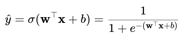
Here:

• hat{y} represents the predicted probability that the output is 1.

• sigma(.) is the logistic (sigmoid) function, which maps any real-valued input to the range (0, 1).

• w is the parameter vector (weights).

• x is the feature vector of the input.

• b is the bias term (also referred to as the intercept).

Since we interpret hat{y} as a probability, a threshold (commonly 0.5) is typically used for classification: if hat{y} >= 0.5, predict class 1; otherwise, predict class 0. Despite this discrete prediction step, the training process is based on continuous parameter estimation—hence a “regression” approach.

Optimization Using Maximum Likelihood

To estimate the parameters w and b, Logistic Regression maximizes the likelihood of observing the given training data. Equivalently, we minimize the negative log-likelihood. This maximization/minimization is fundamentally similar to many regression-style fits where we attempt to find optimal coefficients by solving an optimization problem.

Below is the typical log-likelihood function for N training examples, which we typically turn into a negative log-likelihood (loss) and minimize:

Here:

• y_i is the true label for the i-th sample (0 or 1).

• hat{y}_i is the predicted probability for the i-th sample given parameters w and b.

• We usually convert this into a loss function J(w, b) = -ell(w, b) and minimize it using gradient-based methods such as Gradient Descent.

This framework of “fitting” or “estimating” coefficients to minimize a continuous cost is characteristic of regression. That is the core reason we refer to it as regression. After training, we still treat the final output as a probability and classify accordingly, but mathematically and statistically, the process is a regression on the log-odds.

Practical Implementation Aspects

In practice, Logistic Regression is implemented in libraries like scikit-learn, PyTorch, or TensorFlow by specifying a loss function (often binary cross-entropy, which is the negative log-likelihood under Bernoulli assumptions). The optimization routine is almost identical to other regression-based models, except that the predicted value is the probability of belonging to class 1. Below is an outline in Pythonic pseudocode:

import torch
import torch.nn as nn
import torch.optim as optim

# Suppose we have feature_tensor (X) and label_tensor (y)
# w is the weights, b is the bias

class LogisticRegressionModel(nn.Module):
    def __init__(self, input_dim):
        super(LogisticRegressionModel, self).__init__()
        self.linear = nn.Linear(input_dim, 1)  # w, b implicitly included

    def forward(self, x):
        # Outputs probability of class 1
        return torch.sigmoid(self.linear(x))

model = LogisticRegressionModel(input_dim=10)  # example dimension

# Binary Cross Entropy Loss = Negative log-likelihood
criterion = nn.BCELoss()
optimizer = optim.SGD(model.parameters(), lr=0.01)

for epoch in range(100):
    optimizer.zero_grad()
    output = model(feature_tensor)
    loss = criterion(output, label_tensor)
    loss.backward()
    optimizer.step()

This example shows that we define a linear function (a typical regression step) and apply the sigmoid for logistic regression. The main difference is the cost function that calculates the negative log-likelihood rather than a mean-squared error.

Why the Name “Regression”?

The name stems from the historical and statistical background of the method. When the model was first introduced, it was seen as a type of regression on the transformed target variable (the log-odds). The output is modeled through a linear function, which is standard in regression tasks. The logistic function simply ensures the output remains in [0, 1], which aligns with the probabilistic interpretation. Technically, once the model parameters are learned, the predicted continuous value is a probability, which gets mapped to a class label. Despite its modern-day usage for classification, the core approach and mathematical underpinnings remain very much in the regression realm.

Common Pitfalls and Misconceptions

A frequent misconception is that Logistic Regression is “just classification” and unrelated to regression. The central point is that the process of fitting parameters to data, using an optimization-based approach, is quite similar to regression models. The “logistic” function does the final squashing into probabilities. Another pitfall is to treat the output as raw linear predictions when the model by design produces probabilities. Failing to interpret the outputs properly can lead to confusion about how thresholds or probability calibration should be handled.

How It Differs from Other Regression Models

Unlike Linear Regression, which can predict values on the entire real line, Logistic Regression confines the predictions to [0, 1] using the logistic function. The cost function is also different: rather than minimizing mean-squared error, we use the negative log-likelihood or cross-entropy loss, which is better suited for binary classification tasks.

Follow-up Questions

Could you explain why we do not just call it “Logistic Classification”?

Logistic Regression involves solving for coefficients that best explain a transformed version of the probability (the log-odds), which is mathematically done by an optimization procedure akin to regression. The classification aspect is a consequence of applying a threshold on the predicted probability. Historically, the name stuck because the underlying technique is more regression-like than a pure classification rule or tree-based approach.

How does the cost function in Logistic Regression differ from that in Linear Regression?

In Logistic Regression, the negative log-likelihood (or binary cross-entropy) is used. This cost function arises from the Bernoulli distribution assumption for the binary labels. In Linear Regression, we typically minimize the sum of squared errors, which follows from assuming Gaussian noise on continuous labels. Hence, the choice of cost function depends on the nature of the dependent variable: binary or continuous.

Why might Logistic Regression be preferred over other classification methods?

Logistic Regression is straightforward, interpretable, and computationally efficient. The learned coefficients have a clear meaning in terms of odds ratios, making it popular in fields such as medical or social sciences, where interpretability is crucial. It also extends to multiple classes through techniques like softmax regression (multinomial logistic regression). For linearly separable data, it can perform quite well and is easier to implement and debug than some black-box methods like deep neural networks.

How does the logistic function help manage extreme predictions?

The logistic function smoothly maps any real value from -infinity to +infinity into the range (0, 1). This provides a probability-like interpretation while also preventing out-of-bounds predictions. Even if the linear term is very large or very negative, the logistic function yields a valid probability, avoiding issues where you might predict invalid probabilities below 0 or above 1.

If I want to handle multi-class classification, can I still use “Logistic Regression”?

Yes. For multi-class tasks, one common approach is Softmax Regression (also known as multinomial logistic regression). Instead of squashing the linear outputs to a single probability for one class, the softmax function is used to produce probabilities for each possible class in a mutually exclusive setting. The underlying principle remains the same: a regression-based approach to optimize parameters using a likelihood-based objective function.

What might happen if the features are highly correlated?

Logistic Regression, like Linear Regression, can suffer when features are highly collinear. The model can exhibit instability in its parameter estimates, leading to large variance in the learned coefficients. Techniques like regularization (L1 or L2) or dimensionality reduction methods can help mitigate this issue. Regularization adds a penalty term to the cost function that discourages overly large weight coefficients, improving generalization and stability of the model.

What if the classes are highly imbalanced?

In cases of severe class imbalance, standard Logistic Regression can be biased toward predicting the majority class. Strategies such as weighting the loss function inversely proportional to class frequency, oversampling the minority class, undersampling the majority class, or using advanced methods like SMOTE can improve performance and prevent the model from neglecting the minority class entirely.

Why do we use Gradient Descent or variants like Newton’s Method to train Logistic Regression?

The cost function for Logistic Regression is not guaranteed to have a closed-form solution for the model parameters (unlike Linear Regression’s ordinary least squares solution). Instead, we rely on numerical optimization methods like Gradient Descent, Stochastic Gradient Descent (SGD), or second-order methods such as Newton’s Method. These algorithms iteratively update the parameters in the direction that reduces the negative log-likelihood until convergence.

All these considerations highlight that while Logistic Regression results in a classification decision, its mathematical underpinning is deeply rooted in regression methodology, which explains the name.