
ML Interview Q Series: Why does maximizing likelihood under normally distributed errors equal minimizing the sum of squared errors in linear regression?

📚 Browse the full ML Interview series here.


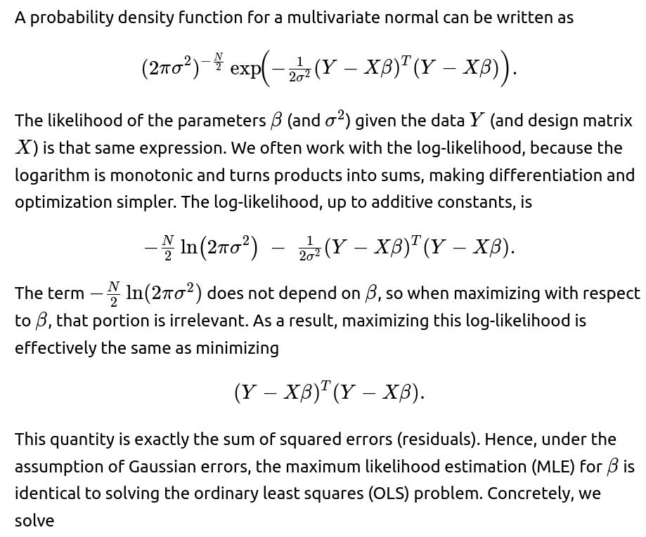

This derivation directly shows that the MLE under a Gaussian-noise model is equivalent to minimizing the sum of squared residuals.
Additional question about the link between MLE and OLS
One might wonder whether there is always a one-to-one match between MLE and minimizing squared errors. In fact, when the error distribution is specifically Gaussian with a constant variance, then yes, ordinary least squares is exactly the same as MLE. If we consider other error distributions (e.g., Laplace, Poisson, or others), then the equivalence changes or disappears. The choice of Gaussian noise is what makes the squared-error minimization a consequence of maximum-likelihood.

Additional question about using the log-likelihood instead of direct likelihood
One may ask: Why do we work with the log-likelihood at all? Directly maximizing the likelihood can be cumbersome because it involves the product of potentially many exponential factors. By taking the logarithm, we transform products into sums, which are simpler to differentiate. Logarithms also avoid underflow issues in numerical computation. Most importantly, the logarithm is a strictly increasing function, so maximizing the log-likelihood yields the same parameter estimates as maximizing the original likelihood function.
Additional question about non-Gaussian error assumptions

Additional question about correlated or heteroskedastic errors

Below are additional follow-up questions
How does multicollinearity affect the parameter estimates in linear regression with normally distributed errors, and what are the potential pitfalls?

How do outliers impact the relationship between maximizing the likelihood and minimizing squared errors, and how might we address them?
In the Gaussian framework, the likelihood is maximized by minimizing squared residuals. Squared errors, however, are highly sensitive to outliers. A single large outlier can have a disproportionately large influence on the objective function, since squaring an already large residual amplifies it.
In real data, outliers can arise from genuine extreme values, measurement errors, data-entry mistakes, or other anomalies. If outliers are due to measurement or data-processing errors, it might be appropriate to remove or correct them. However, if they are legitimate data points, one must carefully decide how to handle them.

What happens if the size of the dataset is smaller than the number of parameters to be estimated, and how does this affect maximum likelihood estimation?

To handle this, practitioners often:
Acquire more data, if feasible.
Use regularization methods (e.g., Ridge, Lasso), which impose additional constraints or penalties on the coefficients to ensure a unique solution.
Reduce dimensionality via feature selection or principal component analysis (PCA) if the original feature dimension is excessively large compared to sample size.
In practice, do we ever deviate from the assumption of εε having constant variance (homoscedasticity)? If so, how is the MLE approach modified?
Yes, real-world data can often show heteroscedasticity, meaning the variance of the error terms can depend on the value of a predictor or some function of the predictor variables. For instance, errors might be larger for higher values of a certain predictor.
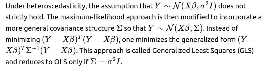
Identifying or estimating the structure of Σ can be challenging. If an incorrect form for Σ is assumed, inference can be biased or inefficient. Sometimes, robust standard errors are employed so that parameter estimates remain valid even when the exact error covariance structure is unknown.
How does numerical precision or very large datasets impact the solution of maximum likelihood via least squares, and what strategies help address these issues?

Could the maximum likelihood estimate under Gaussian errors still be biased, and in what scenarios might bias arise?
The OLS or Gaussian-based MLE estimator for β is typically considered unbiased in the classical linear regression setting if the model is specified correctly (the true data-generating mechanism is linear, errors have zero mean, etc.). However, bias can creep in if:
The model is misspecified (e.g., relevant variables are omitted, or the relationship is not truly linear).
There is measurement error in the predictors or response.
There is data leakage or a non-random sampling procedure that skews the data distribution (selection bias).
Regularization is introduced (e.g., Ridge or Lasso), which shrinks coefficients, thereby introducing some bias in exchange for reduced variance and improved generalization.
Thus, while the unregularized MLE for a correctly specified linear model with Gaussian i.i.d. errors is unbiased in theory, real-world complications (such as omitted variables or measurement noise in X) can introduce biases.
What if the true data generation mechanism is non-linear? Do we still benefit from a linear MLE model?
A linear regression model assumes a linear mapping from features X to the response Y. If the true process that generates Y from X is significantly non-linear, the linear model will systematically fail to capture certain relationships, resulting in a biased and possibly high-variance estimator.
Potential ways to handle this include:
Introducing polynomial or interaction terms to capture non-linearities, effectively enlarging the feature space (still linear in the expanded features, but non-linear in the original sense).
Switching to more flexible models (e.g., kernel methods, neural networks, decision trees) to capture complex relationships. However, these more flexible methods often require careful regularization or pruning to avoid overfitting.
Employing model diagnostics to check for patterns in residuals; any clear structure in residual plots can signal that a linear form is inadequate.
How do we handle missing data while using the MLE framework for linear regression?
Many real-world datasets have missing entries in either predictors or the response. If we naively omit any data rows with missing values, we risk losing valuable information (especially if missingness is not random). This can introduce bias and reduce the size of the dataset.
Several strategies include:
Imputation of missing values: mean imputation, regression-based imputation, or more advanced methods such as multiple imputation. Each approach carries assumptions about why data are missing and how best to fill them in.
Maximum Likelihood with incomplete data: employing specialized algorithms like Expectation-Maximization (EM) that iteratively estimate missing data based on current parameter estimates and then update parameter estimates based on these imputations.
Using a Bayesian approach with priors can be helpful when dealing with missing data in a principled manner, but this can be computationally more intensive.
The pitfall is that any imputation approach relies on assumptions about the distribution of missingness. If data are missing not at random (MNAR), standard methods can yield biased parameter estimates.
In real-world use, how do we validate and check the Gaussian assumption for maximum likelihood linear regression?
After fitting a linear regression model under Gaussian assumptions, diagnostics typically involve:
Residual plots: checking for patterns, trends, or heteroskedasticity in the residuals. If the residuals fan out at high predicted values, that suggests a break in homoscedasticity.
Q-Q plots (quantile-quantile plots): checking if the residuals roughly follow a straight line when plotted against a theoretical normal distribution. Deviations from linearity can indicate heavier tails or skewness.
Formal statistical tests (e.g., Shapiro-Wilk test) to check normality, though in large samples, minor deviations might become “statistically significant” but not practically meaningful.
Pitfalls include overreliance on these tests. Data can slightly deviate from normality without invalidating the linear model. Residual-based checks are not perfect and can fail to reveal certain classes of model misspecifications. Nonetheless, significant or systematic deviations from normality might prompt switching to robust or generalized methods.
How do we interpret confidence intervals or hypothesis tests for the regression coefficients under the MLE framework?

However, if the assumptions (normality, homoscedasticity, independence) are violated, these confidence intervals and p-values can be inaccurate. Users should interpret them carefully, perhaps employing robust or bootstrap methods for more reliable inference in less ideal conditions.