ML Interview Q Series: Why is data more sparse in a high-dimensional space?

📚 Browse the full ML Interview series here.

Comprehensive Explanation

Data appears sparse in high-dimensional spaces largely due to an effect often referred to as the “curse of dimensionality.” The intuitive idea is that as the number of dimensions (features) grows, the volume of the space increases so quickly that any fixed amount of data occupies a relatively small fraction of the available volume. Consequently, data points tend to be spread out far from each other, making many conventional techniques (especially those relying on distance measures) less effective.

A key way to see this is by looking at how volume scales with dimension. Consider the volume of a d-dimensional hypersphere of radius r. It is given by the following formula, which highlights how quickly volume grows with dimension:

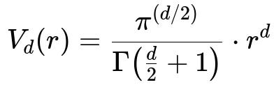
In this expression, d is the dimensionality, r is the radius, pi is the well-known constant (approximately 3.14159...), and Gamma(...) is the gamma function, which generalizes the factorial concept to non-integer values. As d increases, the term pi^(d/2) and r^d can grow very large, causing V_d(r) to expand rapidly. This means that in high dimensions, even a small increase in radius can create an enormous increase in volume, making any fixed number of samples seem sparse since they are spread over a drastically larger region.

Another way to see the sparsity is to consider what “density” might mean in high dimensions. If you are sampling from a hypercube or hypersphere, as you increase the dimensionality, the relative density of points in any particular region (like the center region versus the corners) diminishes if the total sample size remains the same. This leads to the unintuitive scenario that most points lie near the boundary of the hyper-structure, and distance metrics become less reliable in separating or clustering data points.

Beyond the geometric considerations, a more practical perspective is that models often rely on distance-based reasoning—either explicitly in algorithms like nearest neighbors or implicitly in algorithms that measure variance or correlation. When all points are far apart from one another, the notion of “neighborhood” or “local density” becomes difficult to define in a meaningful way. As a result, learning patterns from high-dimensional data often requires larger sample sizes, carefully chosen feature engineering, or dimensionality reduction techniques to mitigate the challenge of sparsity.

What Causes This “Sparsity” Effect More Intuitively

When you move from a low-dimensional setting, such as a 2D space where data might cluster in a small region, to a higher-dimensional one, the points that used to be “close” can grow surprisingly far apart. This is not just about having “more axes”; rather, the geometry itself changes in fundamental ways. The distances become dominated by the largest components, and clusters can spread out so that seemingly similar points in low dimension no longer appear close in a higher-dimensional representation.

How Does Sparsity Affect Model Performance

Models that depend heavily on distance metrics, such as K-Nearest Neighbors or clustering methods, can suffer severely when dealing with sparse data in high dimensions. Distances between data points can become almost uniform, and it becomes challenging to separate signal from noise. Likewise, many machine learning algorithms require a notion of density, neighborhood, or local smoothness, all of which grow difficult to define in a reliable way when the volume of space increases drastically.

Regularization practices, dimensionality reduction, and careful feature selection all become critically important. By reducing the effective dimensionality, we aim to place data points in a more compact representation space where distances and local neighborhoods are more meaningful.

Why Does Volume Concentrate Near the Edges

A subtle aspect of high-dimensional spaces is that volume tends to accumulate near the outer “shell” (or boundary) of a hypersphere rather than near its center. This boundary concentration is another perspective on why data looks sparse: even if you distribute samples throughout the space, many of them end up in regions we might consider “edges,” making inner regions relatively empty. This poses a conceptual obstacle for algorithms that expect data to be dense around certain centers, leading to misinterpretations about distance and similarity.

Practical Consequences in Machine Learning

Training data size requirements grow quickly because to ensure good coverage of the input space, you need exponentially more samples as you add more dimensions. High-dimensional feature vectors often contain redundant or irrelevant features, which can exacerbate the data sparsity problem. Techniques like Principal Component Analysis (PCA), autoencoders, or random projections are commonly used to project data into a lower-dimensional space while trying to preserve the structure and variability of the original data.

Potential Mitigations

In real-world applications, approaches to mitigate sparsity in high-dimensional data can include:

Dimensionality reduction: PCA, t-SNE, UMAP, and autoencoders can reduce the dimensionality of the data while preserving essential relationships.

Feature selection: Domain knowledge to select only the most relevant features can reduce unnecessary dimensions, preventing the model from “diluting” its capacity across many irrelevant axes.

Distance metric learning: Learning more sophisticated distance metrics or kernel functions that capture similarity better in high-dimensional spaces can improve performance.

Regularization: Encouraging sparsity in weights (L1 regularization) or penalizing overly complex models (L2 regularization) can help the model generalize better in the face of limited data for many features.

Why Does Increasing the Number of Dimensions Make Distances Less Meaningful

One of the stark realities of high-dimensional data is that distances between any pair of points often become similar. In other words, the ratio between the closest distance and the furthest distance shrinks. This phenomenon makes it difficult to discriminate between points based on distance measures, undermining techniques like K-Nearest Neighbors or distance-based clustering.

Further Interview-Level Follow-up Questions

How Do We Alleviate the Issues When Using Distance-Based Methods in High Dimensions?

One option is to pre-process the data. For instance, you could reduce dimensionality with PCA or a neural network–based embedding (such as an autoencoder) before applying any distance-based method. This technique helps ensure that points truly close in the feature space remain close in the transformed space. Feature selection can also prune away noisy, irrelevant features that add unhelpful dimensions and hamper distance calculations.

What Are Some Real-World Pitfalls Stemming from High-Dimensional Sparsity?

One pitfall is overfitting: with so many dimensions and so few samples, a model can latch onto spurious correlations that do not generalize. Another pitfall involves interpretability: as dimensions increase, understanding why a certain prediction is made can become more complex. Also, in fields such as recommender systems or text analytics, dealing with extremely sparse vectors is common (e.g., very high-dimensional word embeddings), and naive distance-based methods might not yield good results without careful transformations or specialized similarity measures.

Are There Situations Where High Dimensionality Helps Rather Than Hurts?

Sometimes higher dimensions can help if relevant signals are embedded in those dimensions and the model is capable of uncovering them. Neural network–based representations (like embeddings) can uncover complex relationships across features. However, this advantage typically requires very large datasets and strong regularization to avoid overfitting, and well-designed architectures that can systematically learn useful representations.

By understanding these nuances—both the geometric intuition and the practical mitigation strategies—engineers and data scientists can design robust pipelines that properly handle the challenges of sparse data in high-dimensional settings.

Below are additional follow-up questions

How does high-dimensional sparsity impact the interpretability of models, especially in regulated industries?

High-dimensional datasets often lead to complex models with large numbers of parameters. In regulated fields like finance or healthcare, decision-making processes must be transparent for auditing and compliance. When dealing with sparsity:

• Models such as deep neural networks might become “black boxes.” Interpretability tools (e.g., SHAP, LIME) could struggle if features have sparse correlations. • Even simpler linear models can become unwieldy if they have thousands of coefficients (one per dimension) that are difficult to interpret collectively. • Important edge case: if a single dimension is crucial (e.g., a rare genetic marker in healthcare), it might be masked by the noise in many irrelevant dimensions. Automated feature selection might discard it unless carefully managed.

Sparsity makes it harder to ensure that the model behaves ethically, fairly, or logically from a domain-specific standpoint, so domain experts might have to impose constraints on the model or use specialized regularization that nudges interpretability.

How do generative models (like VAEs or GANs) cope with sparsity in high dimensions?

Generative models aim to learn the underlying distribution of data. In high-dimensional spaces:

• Models such as Variational Autoencoders (VAEs) rely on finding lower-dimensional latent spaces that capture essential features. If data is highly sparse, learning a stable latent representation can be challenging because the generator must cover many possible configurations of the dimensions. • GANs can suffer from mode collapse if certain regions of the space are rarely visited by real samples, reinforcing sparsity. • A pitfall arises when the model devotes too many parameters to rarely populated regions of the space, leading to overfitting and poor generalization. In real-world tasks like image generation, partial solutions include specialized architectures (e.g., convolutional layers that exploit spatial structure) or carefully designed regularization.

The interplay between model complexity and data sparsity demands large training sets or domain-informed priors to avoid producing artifacts or failing to generate diverse samples.

How do distance-based outlier detection methods perform in high-dimensional spaces, and what are possible pitfalls?

Distance-based outlier detection (like k-Nearest Neighbors outlier detection) can become unreliable:

• In high-dimensional spaces, distances may concentrate; nearly all points can appear roughly equidistant from each other. This obscures which points are genuinely “outliers.” • A subtle pitfall: a data point may seem to be an “outlier” in a particular subset of features but not in others; in high dimensions, combining these can lead to contradictory signals about whether it is genuinely unusual. • Edge case: if the dataset has micro-clusters of anomalies (e.g., points forming a small cluster in the corner of the space), a purely distance-based method might mislabel them as normal if the local neighborhood is consistent.

In practice, one often pairs dimensionality reduction with robust outlier detection algorithms such as isolation forests or local outlier factor, ensuring that anomalies remain distinguishable in a more tractable lower-dimensional representation.

When does high-dimensional data call for specialized hardware or distributed computing?

Large-scale, high-dimensional datasets (such as those in genomics, image analysis, or clickstream logs) can require significant computational resources:

• GPU or TPU acceleration is often necessary, especially if matrix operations become huge in dimensional terms (e.g., thousands or millions of features). Memory constraints might become a bottleneck if naive processing attempts to store massive dense matrices in RAM. • Distributed computing frameworks like Spark or Dask can be critical for tasks such as computing pairwise distances. A pitfall is network overhead: transferring large data blocks across cluster nodes can overshadow computational gains if not carefully optimized. • A subtle real-world issue emerges if intermediate transformations balloon the data size (e.g., one-hot encoding with extremely large cardinalities). Careful design of dataflow pipelines to handle partial transformations or on-the-fly calculations may be necessary to avoid saturating memory.

Computational infrastructure planning thus becomes an integral part of the design for modeling high-dimensional data, ensuring that the system can scale appropriately and efficiently.

How do Bayesian methods deal with high-dimensional parameter spaces?

Bayesian approaches define a prior over parameters and then update that prior to a posterior given data. In high-dimensional parameter spaces:

• The prior distribution might become diffuse, making it difficult for sampling algorithms (like MCMC) to converge. If the dimensionality of the parameter space is large, the Markov chain might explore configurations very slowly, leading to extremely long training times. • Another subtlety arises if the likelihood is peaked in a complicated region due to sparsity. The sampler may get stuck in local modes, missing significant areas of the posterior distribution. • A real-world pitfall emerges when practitioners use overly simplistic priors that do not reflect domain knowledge. In high dimensions, this can steer the posterior away from meaningful solutions or cause it to overfit if the data is not sufficient to narrow down the enormous parameter space.

Techniques like Hamiltonian Monte Carlo or Variational Inference can handle higher dimensions more efficiently than basic MCMC, but the curse of dimensionality still demands careful priors, model architectures, and occasionally dimension reduction of the parameter space itself.

How does data augmentation help address sparsity in high-dimensional datasets?

Data augmentation involves artificially creating new examples from existing data:

• In image processing, transformations like random crops, flips, or rotations can expand the effective dataset without requiring new labeled data. In high-dimensional tabular data, augmentation is trickier, as naive perturbations might not preserve real-world relationships among features. • When data is sparse, well-chosen augmentations can fill “gaps” in feature space, improving model robustness. A critical pitfall is generating unrealistic samples that mislead the model, particularly in sensitive domains like healthcare or finance. • An edge case arises if the augmentation overrepresents certain regions of the feature space, skewing the learned distribution. Balancing realism and diversity is essential.

Therefore, augmentation in high-dimensional settings must incorporate domain expertise to generate plausible variations that genuinely help reduce the detrimental effects of sparsity.

How do you determine if your dimensionality reduction is losing critical information?

Dimensionality reduction can mask essential details if not done carefully:

• One way is to measure reconstruction error: for methods like PCA or autoencoders, compare the reconstructed data against the original. A low mean squared error might indicate minimal information loss, but not always—it depends on which features matter most for the task. • For classification tasks, track predictive performance (e.g., accuracy, F1-score) before and after dimension reduction. If performance drops dramatically, it suggests that the reduced features lost discriminative power. • A subtle edge case arises if the data has rare but critical features (e.g., a small set of outlier points that are crucial for detecting fraud). Common dimensionality reduction methods might discard such outliers, as they contribute minimally to global variance.

Hence, it is not enough to evaluate reconstruction error alone; you must consider domain-specific performance metrics and outlier sensitivity to ensure that essential information is preserved.

What steps can be taken if domain constraints forbid feature removal or dimensionality reduction?

Certain regulations or domain requirements may mandate retaining all raw features:

• One strategy is advanced regularization, using methods like elastic net or group sparsity to reduce model complexity while formally keeping all features in the pipeline. Such methods encourage the model to distribute or constrain weights, focusing only on the most relevant parts. • Kernel-based methods can sometimes map data into a space that handles redundancy, but the high-dimensional kernel computations might become expensive. Careful sampling or approximations (like the Nystroem method) may be needed. • Another subtle scenario arises when the domain demands certain interpretability constraints—for example, each feature might represent a legal or regulatory factor. You could use interpretable model classes (like generalized additive models) that handle all features but still allow some clarity into how each influences the output.

Balancing the real-world requirement to keep every dimension with the practical necessity to manage sparsity often involves creative modeling, advanced regularization, and thorough validation.

How can one detect and address hidden correlations in high-dimensional data?

When dealing with many features, hidden correlations or multi-collinearity can inflate the effective dimensionality:

• One approach is calculating correlation or covariance matrices and examining them with methods such as PCA to find highly correlated feature blocks. A subtle pitfall is that not all correlations are linear; feature pairs might appear uncorrelated in linear terms but still have non-linear relationships. • In real-world datasets (like financial time series), correlation might be dynamic and shift over time. A static correlation analysis could overlook scenario-specific patterns. • Modeling techniques like factor analysis or partial correlation networks can reveal underlying structures. Another strategy is domain-driven grouping of features so that collinear or related ones are combined or replaced with latent factors.

Identifying and mitigating these hidden correlations is essential, as ignoring them can lead to models that overfit or misinterpret the relative importance of features.

How do you verify that your high-dimensional model generalizes to unseen scenarios?

Ensuring generalization requires more nuanced validation strategies:

• Standard cross-validation can still be effective, but the partitioning strategy must be robust. In some edge cases, random splits might not reflect real-world distributions if specific rare classes or subpopulations exist. Stratified splitting or time-based splitting (in temporal data) can help preserve important structures. • Monitoring generalization across subgroups is crucial if the dataset is high-dimensional and heterogenous. A model might perform well on average but fail miserably on niche subsets (sparsely populated corners of the feature space). • In real-world tasks like medical diagnostics, prospective validation (evaluating on data collected after the model has been finalized) can expose how the model handles new shifts in distribution or unknown confounders.

Thorough validation protocols, combined with stress testing on rare but important sub-populations, help confirm whether the model truly handles the dimensional complexity rather than overfitting.