
ML Interview Q Series: Why is re-scaling gradient updates by class frequency more effective than class-weighting in cross-entropy?


📚 Browse the full ML Interview series here.
Hint: It can stabilize updates by normalizing gradient magnitudes.
Comprehensive Explanation
When dealing with highly imbalanced datasets, it is common to assign higher weights to the minority classes so that errors on these classes contribute more to the overall loss. This approach is often implemented through class-weighted cross-entropy, where the cost function is multiplied by some factor proportional to the inverse frequency of each class. However, simply multiplying the cross-entropy loss for minority classes by a large factor can lead to very large gradients that may destabilize optimization. Re-scaling the cost function’s gradient updates by class frequency (rather than just weighting the loss itself) can be more stable, because it directly controls how much each class influences the gradient magnitudes during backpropagation.
One way to illustrate this in more concrete terms is through the weighted cross-entropy function for binary classification:
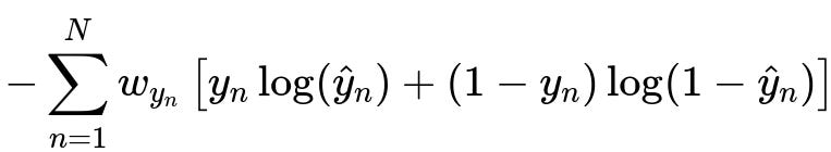
Here, y_n is the ground-truth label for sample n (0 or 1), hat{y}n is the predicted probability that the label is 1, and w{y_n} is the weight for the class to which sample n belongs. In typical class-weighting, w_{y_n} might be set to something like total_samples/(number_of_classes * samples_in_class_of_y_n). In heavily skewed scenarios, if w_{y_n} for the minority class is large, then gradient updates on that class may become disproportionately large, causing unstable updates, especially if the optimizer’s learning rate is not carefully tuned.
Re-scaling the gradients themselves can help mitigate this. Instead of only scaling the final cross-entropy calculation, one can normalizing the gradient update so that, for each class, the contribution to the parameter updates is balanced. This approach effectively controls the norm of the gradient for each class and can prevent extremely large updates while still giving minority classes an appropriately higher influence compared to majority classes.
Another advantage of re-scaling at the gradient level is flexibility. One can dynamically adjust these re-scaling factors during training to adapt to changing distributions (for instance, in streaming data scenarios). This can lead to a more controlled optimization trajectory, reducing the risk of overshooting minima when the minority class gradient is very large.
In practical terms, large deep learning frameworks allow for such re-scaling. One might implement it by manually computing the class-based gradient contributions in a custom loss function and then normalizing or re-scaling it after computing the raw gradient but before performing the parameter update step. This ensures each class’s gradient magnitude does not explode or vanish simply due to a large or small weighting factor.
Practical Example in PyTorch
import torch
import torch.nn as nn
import torch.optim as optim

class CustomWeightedCELoss(nn.Module):
    def __init__(self, class_weights):
        super().__init__()
        self.class_weights = torch.tensor(class_weights, dtype=torch.float)

    def forward(self, logits, targets):
        # Standard cross-entropy
        ce_loss = nn.functional.cross_entropy(logits, targets, reduction='none')

        # Multiply each sample by its corresponding class weight
        # Example: class_weights is an array/list with entry per class
        weighted_loss = self.class_weights[targets] * ce_loss

        # Instead of simply taking the mean, we can re-scale the gradient updates
        # by normalizing the weighted loss
        sum_weights_per_batch = torch.sum(self.class_weights[targets])
        scaled_loss = weighted_loss.sum() / (sum_weights_per_batch + 1e-8)

        return scaled_loss

# Example usage
model = nn.Linear(10, 2)  # Simple binary classifier
criterion = CustomWeightedCELoss(class_weights=[0.2, 0.8])  # Just an example
optimizer = optim.SGD(model.parameters(), lr=0.01)

# Dummy inputs and labels (batch_size=5, input_dim=10)
inputs = torch.randn(5, 10)
labels = torch.randint(0, 2, (5,))

# Forward pass
logits = model(inputs)
loss = criterion(logits, labels)

# Backward and update
optimizer.zero_grad()
loss.backward()
optimizer.step()
In this example, the scaled_loss divides the sum of weighted losses by the sum of the class weights for that batch. This keeps the effective gradient in a more controlled range, avoiding extremely large updates even when the minority class weight is high.
Deeper Reasoning
If we only weight the loss itself, we may inadvertently amplify the gradient for rare classes without bound, especially if there is a mismatch between the learning rate and the magnitude of the weighted loss. By normalizing or re-scaling gradients, we ensure that no single batch or class can skew the parameter updates disproportionately. This addresses issues like:
High variance in gradient norms between classes that differ by orders of magnitude in frequency.
Difficulties in optimizer hyperparameter tuning, since the learning rate might need constant adjustment to accommodate very large or very small gradient magnitudes.
Overfitting minority examples if the weighted cross-entropy is too large for the minority class; normalizing the gradient helps alleviate abrupt parameter shifts that degrade generalization.
Potential Follow-Up Question: How does gradient re-scaling compare to other methods like focal loss in handling class imbalance?
Focal loss applies a factor that down-weights well-classified examples, focusing training on hard, misclassified examples. Re-scaling the gradient by class frequency focuses on the issue of label imbalance rather than example-specific difficulty. Both can complement each other. For severely skewed data, you might combine class re-scaling with a focal-like mechanism to address both problems at once.
Gradient re-scaling is usually more direct and addresses the fundamental problem of gradient explosion or neglect due to imbalance. Focal loss can help improve the model’s focus on hard examples even within the same class, providing a different axis of improvement.
Potential Follow-Up Question: Are there specific optimizers that handle large gradient variations better than others?
Optimizers like Adam or RMSProp adapt the learning rate for each parameter based on historical gradient magnitudes. They can handle large variations to a degree, but extreme imbalance can still cause poor convergence if the raw gradient magnitudes vary too widely. Gradient re-scaling is helpful regardless of the optimizer choice because it uniformly controls the scale of the updates before the optimizer’s adaptive mechanisms kick in.
Potential Follow-Up Question: Could data sampling strategies replace or reduce the need for gradient re-scaling?
Upsampling the minority class or downsampling the majority class can help the model see more balanced batches. However, upsampling may lead to overfitting on the minority class, and downsampling can discard valuable information from the majority class. Gradient re-scaling can be seen as a more continuous approach: rather than changing the data distribution, it changes how the model reacts to each example’s error signal. Both strategies can be combined for potentially better results, depending on the dataset and problem constraints.
Potential Follow-Up Question: How might we decide on the magnitude of the gradient re-scaling factors?
In practice, a popular choice is to use the inverse frequency of each class. Another strategy is to rely on hyperparameters tuned via cross-validation, searching for multipliers that optimize a suitable metric (e.g., F1 score or AUROC). Some practitioners also experiment with dynamically updating these factors during training to adapt to changing class distributions or partial labeling scenarios. The key is to measure the effect on validation data and ensure that the scaled gradients do not lead to harmful oscillations.
Potential Follow-Up Question: Does gradient re-scaling always help with every model architecture?
Complex architectures like large transformers, CNNs, or RNNs can still benefit from balanced gradient magnitudes when classes are imbalanced. However, if the dataset is only mildly imbalanced or if the imbalance is actually reflecting real-world prevalence that we do not want to distort, heavy re-scaling might degrade performance. In those cases, a moderate or no re-scaling might be more beneficial. It is important to monitor metrics that reflect the real-world objective to decide how much or how little re-scaling to apply.
Below are additional follow-up questions
What if the dataset has multi-class imbalance instead of just binary imbalance?
When there are more than two classes, each with its own degree of imbalance, one might want to assign a different gradient re-scaling factor for each class. Simply weighting the loss for each class independently could work, but the overall gradient contributions can still become unbalanced if, for example, two minority classes have extremely different frequencies. Additionally, in a multi-class problem, errors across certain subsets of classes may be more critical for the final performance metric, so it is important to monitor metrics that capture each class’s performance individually (e.g., macro-averaged F1 or per-class precision and recall).
Pitfalls arise if one or two classes in a multi-class setting are extremely rare. If their re-scaling factor is too high, the model might over-commit resources to fitting those rare classes, which in turn can degrade performance on more common classes. Another edge case is if some classes are not just rare but also inherently harder to classify; gradient re-scaling can amplify or mask that difficulty if not carefully tuned. Hence, consider a balanced approach: set initial re-scaling factors based on inverse frequency, but then validate and adjust based on multi-class confusion matrices and overall performance.
Could extremely large re-scaling factors for very rare classes cause overfitting?
Yes. When a class is extremely rare and is given a very large re-scaling factor, the model might learn to fit those few examples too aggressively. Overfitting manifests in training metrics that look good for the minority class but fail to generalize. This is especially problematic if the minority class examples are not representative of all possible examples from that class.
In practice, monitor validation metrics for both the minority class and the majority classes. If you notice that the minority class achieves very high recall on the training set but very low precision on the validation set, or if the overall validation performance starts dropping, it is a sign of potential overfitting. You might consider reducing the re-scaling factor or exploring data augmentation to increase the effective sample size for the minority class.
How does gradient re-scaling help if the minority class has more complex variability?
Sometimes a minority class has higher intra-class diversity (i.e., the data points belonging to that class differ wildly from each other), making it harder to learn a robust representation. Even if we re-scale the gradients, the model might not adequately capture all the variations in that minority class. Re-scaling ensures more weight is given to that class’s loss signals, but it does not guarantee better feature representation if the class itself is more variable.
A pitfall here is assuming that re-scaling alone is enough to handle classes with higher complexity. If complexity is the main issue rather than the raw frequency, other approaches—such as more expressive architectures, specialized feature engineering, or collecting more diverse training examples for the complex class—can often have a greater impact than re-scaling alone. Still, re-scaling does help the optimizer focus more on those complex examples than it otherwise would.
Does gradient re-scaling adapt well if the imbalance changes over time?
In real-world scenarios, class distributions can shift (e.g., in fraud detection, the fraud rates can change over seasons or years). If you rely on static re-scaling factors determined by a single training set, the model might become less effective once the distribution shifts significantly. One approach is to monitor incoming data and dynamically update the re-scaling factors based on a rolling estimate of class frequencies.
A subtle issue is ensuring that these dynamic changes do not make training unstable. If the distribution shifts often, the re-scaling factor for one class might jump repeatedly. To handle this, you can implement a smoothing or exponential moving average approach on the estimated frequencies, so that re-scaling factors adjust gradually rather than abruptly. This helps the model adapt to shifting distributions without sudden, destabilizing changes in gradient magnitude.
How do we ensure gradient re-scaling does not conflict with other normalization layers?
Normalization layers (e.g., batch normalization, layer normalization) are designed to keep activations or feature distributions stable across layers. Gradient re-scaling operates at the loss level, effectively adjusting the error signal before it propagates back through the layers. In principle, they do not conflict directly, but there are some subtle considerations:
If your re-scaling factor becomes large enough, it might drastically influence the effective range of gradients flowing back into earlier layers, potentially saturating or overwhelming the benefit of normalization layers. This can happen especially in deeper networks. It is helpful to track the distribution of gradient norms after re-scaling to confirm that you are still within a stable range.
In edge cases, particularly large re-scaling might lead to issues like vanishing or exploding gradients if the rest of the network architecture is not designed to handle them. Hence, careful tuning of re-scaling factors alongside your chosen normalization technique can avoid these extremes. Checking histograms of gradients in a tool like TensorBoard or similar can reveal if normalization layers are being saturated by huge gradient flows in minority-class examples.
Are there situations where separate specialized models might outperform a single re-scaled model?
In some cases, especially if a minority class represents a very different distribution or subtask, training a separate model (or an ensemble of models) may be more efficient than trying to coax a single model to handle everything. For example, in anomaly detection, the minority class might require specialized methods that focus on one-class or anomaly detection principles.
If you suspect the minority class requires a substantially different set of features or if it is extremely rare, a dedicated model that uses a specialized architecture may outperform a single universal model with gradient re-scaling. The pitfall is that managing multiple models can increase system complexity. Additionally, you lose the synergy of multi-class learning where shared feature representations might benefit from seeing all classes together. The decision typically comes down to empirical performance comparisons and resource constraints.
How does gradient re-scaling scale to very large datasets with extreme class imbalance?
When you have an extremely large dataset (say, millions of examples) and one class is present in only 0.01% of the data, even small changes in the re-scaling factor can lead to a large shift in gradient distribution. In large-scale settings, computational cost can also become an issue when re-scaling requires more advanced data handling or dynamic updates.
Furthermore, in a massive dataset, minority classes still have many examples in absolute numbers, so the advantage of re-scaling might be different from a small dataset scenario. You might still end up with enough minority examples that re-scaling is less crucial. Alternatively, if the minority class is extremely small in absolute terms (e.g., extremely rare catastrophic events), then advanced oversampling or specialized anomaly detection might be more effective than pure gradient re-scaling.
It is important to note that at large scale, naive re-scaling can lead to numerical instability: summations or averages in floating-point may become large, causing floating-point inaccuracies. Regularly monitoring your training loss distribution and gradient norms is vital in large-scale systems to ensure you are not hitting floating-point limits or experiencing unreasonably large updates.
What if the model starts to confuse minority examples among themselves after gradient re-scaling?
A subtle real-world issue is when several minority classes exist, each with their own re-scaling factor. The model might start to pay more attention to those classes collectively, but not necessarily distinguish them well from each other. This phenomenon is sometimes referred to as confusion within minority classes. The gradient signals from multiple minority classes collectively may overshadow the majority class signals, but among those minority classes, the model might not have enough capacity or clarity to differentiate them properly.
One solution is to monitor a per-minority-class confusion matrix. If it is discovered that classes within the minority group get confused with each other, you may need to allocate separate re-scaling factors or even separate specialized heads in a multi-task approach. Another potential solution is to incorporate additional domain knowledge or features that help distinguish among these minority classes rather than just ramping up the gradient magnitude.
How do we debug if gradient re-scaling leads to unstable training?
Unstable training typically appears as large fluctuations in the training loss or significant oscillations in validation metrics. Sometimes, the model parameters may diverge entirely, causing NaN losses. To debug:
Check Gradients: Inspect the distribution of gradients for each batch. If some batches lead to abnormally large gradient values, it suggests the re-scaling factor might be too high.
Reduce Learning Rate: Occasionally, a lower learning rate can help mitigate the effect of higher gradient magnitudes.
Adjust Re-scaling Factor: Lower the re-scaling factor for severely imbalanced classes. Iteratively refine it and observe if training stabilizes.
Implement Gradient Clipping: If you must keep the re-scaling factors high, gradient clipping (e.g., norm clipping or value clipping) can cap extreme gradient values and preserve stability.
Verify Data: Sometimes, data errors or outliers in the minority class can lead to abnormally large gradient contributions.
A real-world pitfall arises if certain outlier examples in the minority class produce extremely large losses that get inflated by re-scaling. You might address this by investigating potential noise or mislabels in the minority set, or by capping the maximum gradient contribution per sample.
How can we detect whether our gradient re-scaling approach is genuinely improving the model in production?
Often, pure validation metrics do not fully capture real-world requirements. Collecting and analyzing data in the live environment is important to see if the improved minority-class performance translates into better outcomes. For instance, in fraud detection, check real-world detection rates and false positives. If you see a better catch rate of fraudulent transactions without an unacceptable surge in false positives, you can conclude your re-scaling approach is valuable.
In some systems, partial deployment (A/B testing) can help confirm whether the changes from re-scaling produce net benefits. An edge case might be if the minority class is so rare or so costly that you cannot afford a higher false positive rate. In that scenario, you might reconsider the magnitude of re-scaling or look into more fine-grained approaches (like cost-sensitive learning that encodes different misclassification costs explicitly).