
ML Interview Q Series: Why Linear Regression Slopes Differ When Swapping Noisy X and Y

Browse all the Probability Interview Questions here.
We have two variables, X and Y, with Y defined as X plus some normally distributed white noise. If we fit a linear model of Y on X, what will be the coefficient? Then, what happens to that coefficient if we switch things around and run a regression of X on Y?
Comprehensive Explanation
When we say Y = X + noise, we typically mean that Y is generated by taking X and adding some independent random component, often denoted as e (epsilon). This noise term e is assumed to be normally distributed with mean 0 and variance Var(e). The question at hand is about the slope (often termed the coefficient) we get from linear regression in these two scenarios:
Regressing Y on X.
Regressing X on Y.
Below is a detailed breakdown of each case and the underlying mathematics.
Regressing Y on X
We use the simple linear regression setup. In the idealized scenario:
Y = X + e
where e is zero-mean white noise (independent of X). For a simple linear regression of the form:
Y = a + bX
the slope coefficient b (often denoted beta) is:
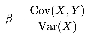
Here, Cov(X, Y) is the covariance between X and Y, and Var(X) is the variance of X. Because Y = X + e and e is independent of X, we have:
Cov(X, Y) = Cov(X, X + e) = Var(X) since Cov(X, e) = 0.
Var(X) is just Var(X).
Hence,
Cov(X, Y) / Var(X) = Var(X) / Var(X) = 1.
So the slope coefficient is exactly 1. Intuitively, since Y differs from X by only a noise term that is uncorrelated with X, the best linear predictor of Y given X (in the ordinary least squares sense) will be Y ≈ 1 · X + constant, with a slope of 1.
Regressing X on Y
If we invert the roles of the dependent and independent variables, we consider:
X = α + γY
and we want to estimate the slope γ from a regression of X on Y. The slope in this regression is:
We have already established that Cov(X, Y) = Var(X). But we must now look at Var(Y). Since Y = X + e, we have:
Var(Y) = Var(X + e) = Var(X) + Var(e),
assuming e is independent of X. Therefore:
Cov(X, Y) / Var(Y) = Var(X) / [Var(X) + Var(e)].
This is strictly less than 1 because Var(X) + Var(e) > Var(X). As a result, the slope γ from the regression of X on Y is:
X = α + (something less than 1) * Y.
In other words, if you swap the roles of X and Y in the regression, the slope shrinks towards zero instead of being 1. This arises because now Y appears in the model as a regressor but also contains noise, so the regression model interprets part of that variation in Y as unreliably predicting X.
Summary of the Two Regressions
• Y on X: The slope is 1. • X on Y: The slope is Var(X) / (Var(X) + Var(e)), which is a number strictly less than 1 (assuming e is non-zero noise).
This asymmetry highlights a critical property of ordinary least squares: the slope you get by regressing Y on X is not simply the reciprocal of the slope you obtain by regressing X on Y when one of the variables includes an added noise component.
Potential Follow-up Questions
Why isn’t the slope in the X-on-Y regression the reciprocal of the slope in the Y-on-X regression?
In simple linear regression, the slope in one direction is Cov(X, Y)/Var(X), whereas in the reverse direction, it is Cov(X, Y)/Var(Y). If Y = X + e, Var(Y) = Var(X) + Var(e). Hence, 1 / [Var(X)/(Var(X) + Var(e))] = [Var(X) + Var(e)] / Var(X), which is strictly greater than 1. Meanwhile, the slope we found for Y on X is exactly 1. So the two slopes do not end up as reciprocals; OLS regression is not symmetrical when the regressor includes noise.
How does measurement error in X (instead of Y) change the conclusions?
In the original setup, Y = X + e, the noise is in Y. If the noise instead were in X, you would similarly get a slope attenuation effect in the Y-on-X regression. Specifically, if X = true_X + e, regressing Y on X would yield a slope smaller than the true slope. The main principle is: When the regressor has measurement error, the OLS slope is biased toward zero (often referred to as “attenuation bias”). When the dependent variable has measurement error that is independent of the regressor, the slope does not suffer from the same bias.
What if both X and Y have noise?
If X and Y both have their own separate noise terms, the relationship becomes more complicated. In such a case:
Regressing Y on X will produce a slope that might be biased if X’s noise correlates with Y’s noise or if X’s measurement error is significant.
Regressing X on Y also might be biased in the opposite direction, especially if Y includes noise. Real-world data often includes measurement errors on all variables, so advanced methods like errors-in-variables models, instrumental variables, or structural equation modeling may be used to deal with the bias.
Could an instrumental variable approach fix the bias?
An instrumental variable (IV) can help if you suspect measurement error in X (or Y). The instrument must be correlated with the potentially mismeasured variable but uncorrelated with the noise. The IV estimation can give an unbiased estimate of the true coefficient. However, identifying a valid instrument that satisfies these conditions can be difficult in practice.
In practice, how do we decide which variable should be X and which should be Y?
Strictly from a regression standpoint, one typically chooses the variable that is more reliably measured or that is truly the “predictor” as the regressor (X). Also from a domain knowledge perspective, you might know which direction of causality or association makes more sense: it is standard to place the hypothesized cause as X and the effect or outcome as Y. But if your goal is purely to measure correlation rather than a causal slope, correlation is symmetric. Regression slopes, on the other hand, are not symmetric when noise is present in the variables.
What if we only want to quantify how well X and Y move together rather than a causal relationship?
If you merely want to measure the linear association, you would consider the correlation coefficient, which is symmetric with respect to X and Y:
cor(X, Y) = Cov(X, Y) / [sqrt(Var(X)) × sqrt(Var(Y))].
This metric stays the same regardless of whether you think of X or Y as the predictor. But as soon as you perform a linear regression to predict one variable from the other, you are not measuring correlation alone; you are estimating a slope that depends on which variable is considered the independent variable in the model.
Could we have deduced that the slope is less than 1 when regressing X on Y without any math?
Yes. By intuition: Because Y = X + some extra noise, Y tends to vary more than X. So if you try to use Y to predict X, you are incorporating that excess variability from noise. The regression picks a slope smaller than 1 to compensate for the fact that Y contains fluctuations not strictly tied to X. That is the classic “regression dilution” or “attenuation” phenomenon.
Those are the key points that address why the slope is 1 when Y is regressed on X (given Y = X + e and e is independent noise), and why the slope is smaller than 1 if we switch and regress X on Y. Both the formal math derivation and an intuitive understanding are important in any interview discussion on regression with added noise.
Below are additional follow-up questions
What if the noise is not normally distributed?
Even though ordinary least squares (OLS) often assumes normality of errors for certain statistical tests and confidence intervals, the slope estimates themselves remain unbiased under more general conditions as long as the noise has zero mean and is independent of the regressors. Non-normal noise primarily impacts inference rather than the coefficient’s unbiasedness. For example, if the noise distribution is skewed or has heavy tails (e.g., a Cauchy or Laplace distribution), the point estimate of the slope is still unbiased if the mean of the noise is zero and it remains uncorrelated with X. However, the standard errors and confidence intervals from standard OLS formulas may become inaccurate. In practice, one might switch to robust standard error estimates or Bayesian methods that allow for different noise distributions. A subtle pitfall is that if outliers occur due to heavy-tailed noise, the regression slope could be heavily influenced by those outliers and might not reflect the “typical” relationship between X and Y.
What if the noise is correlated with X?
If the noise term is correlated with X, the assumption of exogeneity in linear regression is broken. In that case, the OLS estimate for the slope becomes biased and inconsistent. This problem is often described as endogeneity or omitted variable bias. For instance, if Y = X + e, but e itself increases when X increases (positively correlated), then part of the variation in Y that appears to come from X is actually being driven by e. This leads to an overestimate or underestimate of the true coefficient (depending on the sign and magnitude of the correlation). A real-world example is if X is household income and Y is consumption, but the noise includes unobserved variables (e.g., credit access) that are also correlated with income. Analyzing such data without correcting for this correlation leads to distorted slope estimates. The typical remedy is to use methods such as instrumental variables, panel data techniques (if repeated measurements are available), or structural equation modeling to separate the exogenous portion of X from the correlated noise.
What if the variance of X is extremely small or nearly zero?
When the variance of X is very small, it is challenging for OLS to distinguish how Y changes in response to X. Variance in X is crucial for estimating the slope because slope is computed roughly as Cov(X, Y)/Var(X). If Var(X) is near zero, the denominator of that fraction is extremely small, potentially leading to very large and unstable slope estimates. In the pathological case where X has zero variance (i.e., X is constant), you cannot run a regression of Y on X at all because there is no variability in X to explain Y. This scenario can also happen with real-world data that is nearly constant within certain subsets of a population. One pitfall is that even small rounding errors or measurement noise in X can become amplified in the slope estimate, leading to huge confidence intervals or numerical instability. In practice, one should verify that the predictor variable has enough variation to justify the regression model.
How do non-linear relationships impact these results?
When Y depends on X through a non-linear function plus noise, the simple linear regression framework with a single slope no longer fully captures the relationship. For example, if Y = X² + e or Y = log(X) + e, then fitting a linear model Y = a + bX might produce biased estimates that systematically underfit or overfit different regions of X. The question specifically about Y = X + noise yields a slope of 1 only if that linear relationship holds. The presence of non-linearities changes the interpretation of the slope to something akin to an average linear approximation over the range of X. Additionally, the assumption that e is independent of X might remain, but because the model is mis-specified, the slope estimate might not represent the true effect of X on Y at all points. In real-world scenarios, one might test polynomial expansions or transformations of X to better capture the actual Y–X relationship.
What if the data has strong outliers?
Outliers can distort OLS estimates since ordinary least squares minimizes the sum of squared residuals, giving outliers (which have large residuals) a very high leverage in influencing the slope. Even if the true relationship is Y = X + independent noise, a single extreme data point could shift the regression slope away from 1. Outliers may stem from data entry errors, measurement anomalies, or genuinely unusual observations. In practice, it is crucial to diagnose the presence of outliers through residual plots and robust statistics. A robust regression method (e.g., Huber loss, RANSAC, or quantile regression) can reduce the undue influence of outliers. This is particularly important because the scenario “Y = X + e” theoretically places the slope at 1, but real data with outliers might produce a slope significantly different from 1 unless robust methods or careful data cleaning are applied.
What if we are dealing with time series data where both X and Y are evolving over time?
In time series, the assumption of independence between e and X can be violated if both variables exhibit autocorrelation. Even if you have Y = X + e conceptually, if both X and Y follow certain trends or seasonal patterns, the noise might correlate with past values of X or Y, creating additional structure. This can lead to spurious regression or inflated R² values when dealing with trending data. For instance, X could be a random walk, and Y might also be a random walk; simply regressing Y on X might indicate a strong relationship even if none truly exists in a causal sense (the “spurious regression” phenomenon). Specialized techniques such as cointegration tests, differencing, or vector autoregression (VAR) models could be necessary to properly capture the dynamics. Another subtle pitfall arises if the noise accumulates over time or has auto-correlation, further invalidating classical OLS standard errors.
What if the design calls for simultaneous estimation of both equations X = a + bY and Y = c + dX?
Simultaneous equations models arise frequently in economics and other social sciences, where you might have Y = X + e but also X depends on Y in some way, or both are determined by a common underlying process. In such cases, performing two separate OLS regressions can be misleading because each equation’s error term might be correlated with the other dependent variable. A specialized technique, such as Two-Stage Least Squares (2SLS) or System of Simultaneous Equations (e.g., Seemingly Unrelated Regressions, structural equation modeling), is then used. These techniques ensure that the potential endogeneity in each equation is accounted for properly. Failure to handle this can lead to inconsistencies where neither slope estimate reflects the true structural relationship.
How might small sample sizes affect our confidence in the slope?
With very few data points, even if Y = X + e perfectly holds in theory, random variations in the small sample can give slope estimates that deviate substantially from 1. In small samples, the variance estimates of the slope increase, confidence intervals widen, and hypothesis tests lose power. Normal-based confidence intervals (which rely on approximate large-sample behavior) might become misleading if the sample is too small. Moreover, if the noise distribution is not normal, small-sample inference might become even less reliable. One real-world pitfall is overfitting or coincidental patterns in very limited data, causing misinterpretation of the slope. Researchers often use methods like bootstrapping for more robust uncertainty estimates in small samples, but the fundamental limitation remains that with too few data points, the observed slope may differ significantly from the theoretical slope of 1.
How does heteroscedastic noise alter the regression conclusions?
In the classic linear model, noise is assumed to be homoscedastic (i.e., constant variance across all values of X). If noise variance changes with X (heteroscedasticity), OLS can still be unbiased for the slope under certain assumptions, but the standard errors are no longer valid, and any inference (like hypothesis testing or constructing confidence intervals) can be incorrect. Practically, the slope might still center around 1 in the case of Y = X + e, but the distribution of residuals will differ across levels of X, causing inefficient estimates. Specialized methods like Weighted Least Squares or robust standard errors are typically used to correct for heteroscedasticity. In real scenarios, an investigator might find that for large values of X, the noise spikes due to measurement constraints or dynamic range issues, which can drastically inflate the spread of Y around the regression line.
What if Y is bounded or categorical, so it can’t really be expressed as X plus standard noise?
Sometimes the outcome variable Y is restricted (e.g., Y is binary). A direct linear regression with Y = X + e might be conceptually flawed because the distribution of Y is not continuous or unbounded. In that situation, logistic regression or other generalized linear models are more appropriate. Trying to fit a linear model to bounded data can lead to predictions outside the valid range, and the slope estimate might not have a meaningful interpretation of “1” in the sense of Y = X + noise. A subtle pitfall is to forcibly apply linear regression to a variable that is, for example, in [0, 1], which can yield apparently correct slopes in some intervals but systematically fail outside that range. Instead, one should choose a modeling approach consistent with the data type and known constraints.