
ML Interview Q Series: Why might it be necessary to scale or normalize your features before defining a particular cost function,and how does this relate to the geometry of the cost function landscape?


📚 Browse the full ML Interview series here.
Hint: Think about gradient magnitudes and the shape of the error surface.
Comprehensive Explanation
One of the most critical aspects of training many machine learning models, especially those involving gradient-based optimization, is the issue of feature scaling or normalization. When features in the training set have vastly different scales, the resulting cost function landscape can become elongated or skewed. This distorts the geometry of the error surface and makes optimization substantially more difficult. By bringing features to a comparable scale, one can achieve a more "spherical" contour of the cost function, ensuring more balanced gradients and faster, more stable convergence.
A classic example is the mean squared error cost function used in linear regression. The cost function, often denoted by J(theta) for parameters theta, can be written as:
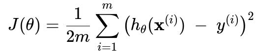
Here, m is the number of training examples, x^(i) is the ith feature vector, y^(i) is the ith target value, and h_{theta} is the hypothesis function (for instance, in simple linear regression, h_{theta}(x) = theta_0 + theta_1 x).
When certain components of x^(i) are on very large scales (e.g., thousands) and others are on smaller scales (e.g., fractions), the contribution of each dimension to the overall gradient may become severely unbalanced. This leads to two main issues:
When performing gradient descent, the parameter updates associated with large-scale features can cause large jumps in the parameter space, while updates for small-scale features move very slowly.
The contours of the cost function can look like a highly stretched ellipse, which slows convergence and often requires a much smaller learning rate to avoid divergence.
By normalizing or standardizing the feature values, each feature dimension tends to have similar ranges. This results in a more balanced gradient magnitude across parameters and typically forms a more spherical cost function contour, allowing a more direct path toward the global minimum. In other words, scaling greatly improves the conditioning of the problem, making gradient-based methods more efficient.
Feature scaling does not alter the underlying relationships in your data. Instead, it puts them on comparable footing, ensuring that certain features do not dominate solely because of their larger numerical values.
Possible Follow-up Questions
What is the difference between normalization and standardization?
Normalization often refers to transforming data so that its values lie between 0 and 1 (or sometimes -1 and 1). A common approach is min-max scaling, where you subtract the minimum value of a feature and then divide by the range (max - min).
Standardization typically involves centering the data around a mean of 0 and scaling to a standard deviation of 1. A common formula would be (x - mean) / standard_deviation. This distribution will have mean 0 and variance 1, and it often handles outliers and different distributions more robustly than strict min-max normalization.
In practical machine learning pipelines, both normalization and standardization are applied for similar reasons: to ensure that no single feature with a large numeric range dominates the cost function or the gradient steps.
Does feature scaling always improve gradient descent convergence?
In a majority of cases, particularly when you have high variance in feature ranges, scaling can dramatically speed up convergence by making the contour shapes more isotropic. However, if all your features already have similar scales or if you are using algorithms relatively insensitive to feature scale (such as decision trees, random forests, or gradient boosting machines), the improvement might be negligible.
In algorithms that rely on distance metrics (like K-Nearest Neighbors or Support Vector Machines with certain kernels), feature scaling is almost always necessary to prevent features with larger numerical ranges from disproportionately influencing distance computations or kernel similarity.
How does feature scaling interact with regularization?
Regularization terms like L2 (ridge) or L1 (lasso) apply penalties to parameter magnitudes. If your features are not scaled, parameters associated with larger scaled features might be penalized more or less in unexpected ways, which can skew the penalty toward certain dimensions. Once features are on a similar scale, the regularization term penalizes each dimension more consistently and fairly.
Can adaptive learning rate optimizers solve the scaling problem?
Methods such as AdaGrad, RMSProp, and Adam adjust the learning rate for each parameter. These optimizers can partially alleviate issues with poorly scaled data by applying per-parameter learning rates. However, they are not a complete substitute for proper feature scaling. Data that is wildly out of scale can still present difficulties during initial optimization steps, and even advanced optimizers tend to perform better when features are at least somewhat standardized.
When could improper scaling cause numerical instability?
In extreme cases—say, a few features are on the order of 10^9 while others are on the order of 10^-3—operations within the cost function or gradient calculations can cause overflow or underflow in floating-point computations. Scaling your data to a moderate numeric range reduces the risk of these numerical issues, which is especially crucial for deep learning frameworks where large intermediate values can cause gradient explosions or vanishing gradients.
How do you handle categorical features when scaling?
Ordinal features (those with a natural ordering) can sometimes be scaled if the numeric distance between categories has a real meaning. However, purely nominal categorical features (like color: red, green, blue) are often one-hot encoded or handled by embedding vectors in neural networks. After one-hot encoding, scaling usually does not apply because those columns take 0 or 1 values. In embeddings, the learned weights automatically scale as needed, although it is sometimes beneficial to initialize them in a small range.
Is feature scaling required for tree-based methods?
Ensemble methods based on decision trees (such as random forests or gradient boosting) tend to be scale-invariant. Tree splits occur according to orderings and thresholds, not absolute distances, so scaling does not usually improve their performance. Nevertheless, if you combine tree-based methods with linear models or other distance-based models in the same pipeline, it can be beneficial to scale your numeric features for the models that depend on absolute distances.
Could unscaled features hide real structure in the data?
Sometimes large magnitudes in certain features reflect genuine importance. If a feature naturally spans a large numeric range and truly dominates the target prediction, scaling might initially appear to degrade the direct interpretability of that feature. However, most algorithms still discover that feature’s importance through the model’s parameters or splitting criteria. If interpretability is crucial, you can always track parameters or feature importances and then transform them back into the original scale for analysis.
How does one decide when to scale features in a production ML pipeline?
As a practical rule, always start with scaling or standardizing numeric features if you are using a gradient-based, distance-based, or neural-network-based method. Evaluate performance with and without scaling in a validation setting. If you see an improvement in convergence speed or metric performance, keep the scaling step. If there is no difference, you can drop it, but be mindful of any edge cases or changes in the data distribution over time. For new features or distribution shifts, re-check whether scaling remains appropriate or if you need to adapt the scaling approach.
In summary, scaling ensures more uniform gradients, prevents certain features from overshadowing others, and leads to a more stable and efficient optimization process. This manifests as a simpler and often more symmetric shape of the cost function landscape, enabling gradient-based optimizers to converge more quickly and reliably.
Below are additional follow-up questions
What if different features require different scaling methods in the same dataset?
Sometimes a dataset has features that exhibit widely varying types of distributions or serve different roles in the predictive model. One subset of features might be best served by min-max normalization, especially if you want values confined to [0,1], while another subset might be better served by standardization (subtracting mean and dividing by standard deviation). Deciding on a per-feature basis can improve performance if done correctly but can also introduce complexity and potential pitfalls.
When features are scaled differently, you need to ensure your pipeline consistently applies the correct transform to each feature at both training time and inference time. For example, you might store separate scaling parameters for each group of features, which increases risk for human error if these parameters get mixed up. Another subtle risk arises when combining the outputs of differently scaled features in subsequent layers or distance metrics; you must ensure that the model architecture or subsequent transformations can handle these heterogeneous scaled ranges. In practice, you might track performance metrics using cross-validation to confirm whether mixing multiple scaling approaches actually helps.
How does feature scaling interact with dimensionality reduction methods like PCA?
Dimensionality reduction methods, such as Principal Component Analysis (PCA), are heavily influenced by the variances of individual features. If features are not scaled, those with larger numeric ranges can dominate the principal components. Standardizing the features so that each has mean 0 and standard deviation 1 often leads to principal components that reflect patterns in the data rather than just variations in scale.
A key edge case to consider is when certain features inherently contain more information because their range legitimately captures greater variance. Blindly scaling those features might reduce interpretability of the principal components. Another subtlety is that some domain knowledge might indicate that certain features should remain unscaled (e.g., a feature measured in decibels or a ratio scale with multiplicative properties). It’s vital to consider domain-specific details: if the large variance in a particular feature is truly significant, over-scaling could mask important structure. Cross-validation is often used to determine whether scaling is beneficial for the overall predictive performance in downstream tasks.
What about outliers when applying scaling or normalization?
Outliers can heavily affect scaling approaches, especially standardization, because both the mean and standard deviation are highly sensitive to extreme values. A single large outlier can cause the standard deviation to become large, making the scaled values of most points very small and compressing most data to a narrow region. Min-max normalization is also impacted by outliers, as an extreme min or max will map almost all other samples to values near the center of the [0,1] interval.
If outliers are genuine rare events that hold critical information, you may want to keep them. However, if they are data errors or non-representative anomalies, you might clip them or remove them before scaling. You can also explore robust scaling methods, such as using the median and interquartile range instead of mean and standard deviation, to reduce the effect of outliers. There is a risk in applying robust scaling, though: if your model is especially sensitive to the absolute distances in the input space (e.g., certain clustering algorithms or distance-based methods), using the interquartile range might shift or shrink distances in a way that misrepresents real domain relationships. Testing different scaling strategies while monitoring performance metrics is key to avoiding these pitfalls.
When might partial scaling (scaling only a subset of features) be a better choice than uniform scaling?
Partial scaling can sometimes be optimal if only a small subset of features exhibits extreme scales. For instance, suppose a dataset has ten numeric features, where eight are already in similar ranges (0 to 1 or 0 to 100), but two features are in the range of millions. Scaling only the outliers can simplify model training without introducing the overhead of applying transformations to every feature.
One potential downside is that partial scaling can introduce inconsistency in how features interact. If your model or downstream processes expect some uniform notion of distance across features (e.g., in kernel methods or in certain neural network architectures), partial scaling might lead to warped or misleading geometry in the feature space. Another subtlety is interpretability: business stakeholders or domain experts who are used to seeing certain features in their original scale may not appreciate that only a subset has been transformed. Documentation and consistent naming conventions can mitigate confusion.
Are there domain-specific reasons not to scale certain features?
Certain features have physically meaningful scales that experts may want to preserve. For instance, in medical imaging or sensor readings, specific amplitude ranges can indicate clinically significant thresholds or safety margins. Arbitrarily altering that scale might risk obscuring domain knowledge. Alternatively, some legal or regulatory requirements demand that raw measurements be stored and used in their original form. Also, in financial applications, ratio-based transformations or log transforms might be standard practice rather than a typical linear scaling.
You must weigh the benefits of algorithmic performance against potential consequences of losing domain interpretability or violating domain-specific constraints. Sometimes, domain constraints require partial transformations (e.g., applying logs to certain features but keeping others as raw measurements). In such scenarios, thorough testing with domain experts is essential to confirm that the chosen transformations do not conflict with real-world usage.
How can we handle feature scaling in streaming or online learning scenarios?
In streaming or online learning, new data continuously arrives, potentially shifting the distribution of features over time. A standard min-max scaling or standardization approach that uses only initial training data statistics (e.g., min, max, mean, or standard deviation) could become outdated. As a result, the scaled values might drift or become inaccurate.
One solution is to maintain a running estimate of the mean, variance, min, and max for each feature and periodically update your scaling parameters. This can be done using incremental statistics formulas. However, if a major distribution shift occurs, your older statistics can become obsolete, and the model’s performance may degrade. A delicate balance is required to decide how much weight to give to recent data versus historical data. In critical real-world applications, you might also implement a drift detection mechanism that triggers recalibration or retraining when the distribution changes significantly.
In deep neural networks, when does batch normalization obviate the need for explicit feature scaling?
Batch normalization is a technique applied to intermediate layers in neural networks to normalize the activations. This helps maintain stable gradients and can often reduce the need for explicit feature scaling of the raw inputs. However, batch normalization might not fully replace input-layer scaling. If the raw input has extremely large ranges, early layers may experience numerical instability before batch normalization can mitigate it.
Batch normalization also introduces additional complexity and parameters (i.e., gamma and beta, which rescale and shift the normalized output). These parameters can learn to adjust internal layer distributions, but if your dataset’s inputs are wildly unscaled, the initial forward pass before update steps can still hamper training. Consequently, many practitioners still standardize or normalize the input data when training neural networks, even if batch normalization is used. This can help the network converge faster and reduce the risk of exploding or vanishing gradients in the earliest layers.
How do whitening transformations differ from conventional scaling?
Whitening transformations (e.g., PCA whitening or ZCA whitening) go beyond simple scaling or standardization by also decorrelating features. Instead of merely ensuring each feature has unit variance, whitening attempts to remove covariance between features so that the transformed features become uncorrelated. This can be beneficial for algorithms sensitive to correlated inputs or for certain neural network architectures where decorrelated inputs stabilize the training process.
However, whitening can amplify noise in directions with tiny variance and can lead to overfitting. Whitening also significantly changes the geometry of your data, which might reduce interpretability because the new axes in the whitened space are not the original feature axes. It’s also more computationally expensive: you need to compute the covariance matrix and its inverse square root. Practitioners typically use whitening for tasks such as image processing or specialized neural networks. For many real-world datasets, simpler scaling suffices, particularly if interpretability and ease of implementation are higher priorities.
If data is processed in mini-batches, do we need to rescale for each batch?
In many machine learning pipelines, particularly large-scale deep learning, data is loaded in mini-batches for efficiency. The typical approach is to compute scaling parameters (mean, standard deviation, etc.) on the entire training set (or a representative subset), then consistently apply those fixed parameters to each mini-batch. If the data distribution remains stable, this method is sufficient.
If the distribution in each mini-batch shifts drastically (e.g., you load data from different domains over time), using a single global scaler might lead to poor scaling for certain batches. An alternative approach could be applying batch-wise scaling, but that can cause inconsistent scaling across batches—training may become unstable because the model sees data scaled differently over different iterations. A compromise solution is to carefully shuffle and combine data from different domains or times, so each mini-batch roughly represents the overall distribution. In practice, advanced techniques like batch normalization also help mitigate small variations in the distribution from batch to batch at the hidden layers.
How does feature scaling affect the interpretability of linear model coefficients?
In linear or logistic regression, each coefficient can be interpreted as the change in the predicted value (or log-odds) for a one-unit change in the feature. Once you scale the feature, you alter what a “one-unit” change means, which changes how you interpret the corresponding coefficient. This can be confusing for domain experts who are used to reading coefficients in the original units.
A typical approach to reconcile this is to transform coefficients back into the original scale for reporting. You can multiply the learned coefficient by the feature’s standard deviation (in the case of standardization) or by the range (for min-max scaling), and adjust any intercept accordingly. Alternatively, you can keep the scaled model internally and maintain a separate mapping that clarifies each coefficient’s effect in the original units. In practice, always document the transformations so that any stakeholder looking at the model coefficients understands the reference scale.
By thoroughly addressing these further questions, you can better navigate the nuanced complexities of feature scaling in real-world machine learning scenarios.