ML Interview Q Series: Why might Mean Absolute Error (MAE) be harder to optimize than Mean Squared Error (MSE) in high-dimensional feature spaces, and how could you mitigate those difficulties?

📚 Browse the full ML Interview series here.

Hint: MAE has a flat gradient for small errors, leading to optimization challenges.

Comprehensive Explanation

Mean Squared Error (MSE) and Mean Absolute Error (MAE) are two widely used loss functions for regression problems. They both measure how close predictions are to the true targets but differ in how they penalize errors and in their mathematical properties.

The Core Formulas

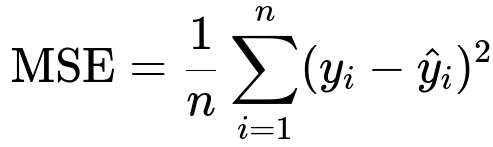
Here n is the number of data points. y_i is the true target for the i-th data point and \hat{y}_i is the predicted value.

Similarly, n is the number of data points, y_i is the true target for the i-th data point, and \hat{y}_i is the predicted value.

Key Differences and Why MAE Can Be Harder to Optimize

MSE penalizes the square of the errors. This gives a gradient that grows linearly with the error term (for example, 2 * (prediction - target) when doing simple gradient-based updates). As a result, MSE is differentiable everywhere, and its gradient smoothly varies.

In contrast, MAE penalizes the absolute value of the errors. For large errors, the gradient can be constant in magnitude (for instance, +1 for positive errors and -1 for negative errors), and at zero error, the absolute value function is not differentiable. In practice, implementations often use subgradients, but these can still be challenging to handle efficiently.

In a high-dimensional feature space, small errors in many coordinates can create plateaus in the MAE landscape. When the absolute difference in each dimension is very small, the gradient can be zero or effectively constant, hindering efficient descent. This is one reason why models using MAE may converge more slowly or get stuck in plateaus compared to those using MSE.

Mitigating the Difficulties

One common solution is to use a loss function that transitions smoothly between MSE and MAE behaviors. Huber Loss is a classic example, where it behaves like MAE (L1) for larger errors but smoothly changes to MSE (L2) behavior for small errors. This allows better gradient flow when the error is small, avoiding the sharp corner at zero that pure MAE has.

Another approach is to use robust optimization techniques that handle subgradients more effectively, such as coordinate descent or specialized solvers built for L1-like objectives. You can also try a two-stage training process: train first with MSE to get in the right ballpark quickly, and then switch to MAE to fine-tune the median-based fit.

Practical Implementation Detail

Below is a small code snippet in Python (using PyTorch) showing how you might experiment with both MAE and MSE losses and potentially use a smoother alternative like Huber Loss for robust optimization:

import torch
import torch.nn as nn
import torch.optim as optim

# Sample data
X = torch.randn(100, 10)  # 100 samples, 10 features
y = torch.randn(100, 1)   # 100 target values

# Simple linear model
model = nn.Linear(10, 1)

# Experiment with different loss functions
mae_criterion = nn.L1Loss()    # MAE
mse_criterion = nn.MSELoss()   # MSE
huber_criterion = nn.HuberLoss(delta=1.0)

# Choose an optimizer
optimizer = optim.SGD(model.parameters(), lr=0.01)

# Example training loop with MAE
for epoch in range(50):
    optimizer.zero_grad()
    predictions = model(X)
    loss = mae_criterion(predictions, y)
    loss.backward()
    optimizer.step()

# You could similarly replace mae_criterion with mse_criterion or huber_criterion

Using Huber Loss (nn.HuberLoss in PyTorch) can significantly mitigate the flat-gradient issue near small errors while retaining the robustness of MAE for large errors.

Possible Follow-up Questions

What is the gradient behavior of MAE and how do implementations handle the non-differentiable point at zero error?

The absolute value function |x| has a constant slope of +1 if x > 0, -1 if x < 0, and is undefined at x = 0. In practice, frameworks use a subgradient concept: if x = 0, they pick any value in [-1, +1]. This can create challenges because a flat or near-flat gradient region might stall optimization. Libraries often define it piecewise, so you get well-defined updates, but it can still cause slower convergence compared to the smoother quadratic error.

How do higher dimensions amplify the challenges of using MAE?

In high-dimensional spaces, the probability of having small but non-zero errors in multiple dimensions is high. Because each dimension might contribute a constant or near-zero gradient, the overall gradient can become very small or inconsistent, causing plateaus. Additionally, data in higher dimensions often exhibits properties (such as sparse relevant directions and many irrelevant ones) that make the constant-slope nature of MAE more likely to lead to slow convergence.

Why might a two-stage training procedure (MSE then MAE) be useful?

Starting with MSE can help the model converge quickly because the gradient is larger and smoothly changes with the prediction error. Once the model predictions are reasonably close to targets, switching to MAE can then refine the fit because MAE is less sensitive to outliers and focuses more on median-like behavior. This approach often yields faster overall convergence than directly training with MAE from the beginning.

What is Huber Loss, and how does it help?

Huber Loss is defined piecewise so that it behaves like MSE for small errors and like MAE for large errors. This helps because near the zero-error region, you get a gradient that changes proportionally with the error (like MSE), avoiding the flat slope of MAE. For large errors, it avoids the extreme penalization of MSE and behaves more robustly, similar to MAE. This smooth transition often yields faster convergence and stability in training.

Can we still use gradient-based methods with MAE despite its non-differentiability?

Yes, and that is typically done using subgradients. Modern libraries handle this internally. The absolute value function has a subgradient of +1 or -1 depending on the sign of the residual. However, you must be aware that even though subgradient methods work, they can be slower to converge, especially in complicated or high-dimensional optimization landscapes.

How do outliers affect MAE vs. MSE?

MSE heavily penalizes outliers because squaring large errors produces very large loss values. MAE has a smaller penalty for large deviations, making it more robust to outliers. That advantage of MAE can sometimes offset the optimization challenges, especially in domains where robustness is a priority.

Are there regularization implications when using MAE (L1) vs. MSE (L2)?

In many contexts, L1 penalty (MAE for errors, or L1 regularization for weights) induces sparsity, while L2 penalty (MSE for errors, or L2 regularization for weights) encourages small but non-zero coefficients. From a regression standpoint, using MAE can help produce models less sensitive to large but sparse errors, while MSE can spread errors more uniformly. The choice depends heavily on the application, the data distribution, and tolerance for outliers.

These discussions reveal the deeper considerations of choosing between MAE and MSE, especially in high-dimensional settings, and the practical workarounds to ensure stable and efficient training.

Below are additional follow-up questions

How does data scaling or normalization affect the behavior of MAE vs. MSE?

MAE and MSE can respond differently to the scale of input data. For instance, if features (or target values) lie on a wide range, MSE can become disproportionately large for errors in the high-scale region because the errors are squared. Meanwhile, MAE, which measures absolute differences, can be more stable but might still converge slowly in high-dimensional spaces if the errors remain uniformly large across many features. In practice, one typically applies standard scalers (like subtracting the mean and dividing by the standard deviation for each feature) or min–max scalers to bring all features to a comparable range. This helps both MSE and MAE because:

• For MSE, you avoid overly large penalty terms caused by a single high-scale dimension. • For MAE, a uniform scale often improves gradient flow so that the constant-slope regions do not overwhelm the optimization in certain dimensions.

A hidden pitfall arises if you apply inconsistent scaling to features vs. targets. If your model output is not scaled the same way as the training targets, either MAE or MSE might lead to skewed gradients. Always confirm that your scaling is consistent for model inputs and outputs where applicable.

What if subgradients are not practical or we want a fully differentiable alternative to MAE?

MAE is piecewise linear and not differentiable at zero error. Deep learning frameworks handle this with subgradients, which is usually sufficient in typical neural network training. However, there are scenarios—like certain specialized optimization methods or hardware accelerators—where subgradient-based updates can be more cumbersome than a smooth gradient.

A common workaround is to replace MAE with a differentiable approximation that closely mimics the absolute value while preserving a smooth derivative. Examples include the soft absolute value functions (like a smoothed L1 norm). Huber Loss can be viewed as one such approach, but there are other variants (e.g., L1 Smooth). These approximations allow the derivative to smoothly transition near zero, avoiding the absolute value’s corner.

A potential pitfall is choosing the approximation’s hyperparameters incorrectly. For instance, a smoothing parameter that’s too large makes the loss behave too much like MSE, losing the robust qualities of MAE. On the other hand, setting it too small may retain the near-flat region around zero error.

How do we handle extremely large datasets with potential outliers if we suspect MAE is slow or gets stuck?

With extremely large datasets, computational efficiency and robustness to outliers become even more critical. Some strategies include:

• Chunk-based or mini-batch optimization: Break down the dataset into manageable batches. This can help measure the gradient more stochastically, sometimes avoiding plateaus from consistently small updates across the entire dataset. • Early outlier detection: If a small fraction of data points are extreme outliers, it can be worthwhile to identify and potentially treat them separately or re-examine data integrity. • Robust losses: Use Huber Loss or a trimmed mean approach where you down-weight extreme outliers. • Parallel/distributed training: Large datasets often require distributed infrastructure. Ensure your framework handles partial gradients consistently.

A key pitfall is ignoring outliers entirely, which might lead to biased models if those outliers are actually systematic (e.g., representing a rarely observed but critical part of the data distribution). Another pitfall is applying heavy trimming or capping, which can lose valuable information.

When might it be valuable to combine MAE and MSE in a single objective?

In some cases, you might form a hybrid loss function like alpha * MSE + (1 - alpha) * MAE. This can offer a compromise: • When alpha is large (close to 1), the objective leans toward MSE. This speeds up early training. • When alpha is small, it becomes closer to MAE, gaining robustness to outliers.

Blending both can be helpful if the dataset has moderate outliers but not enough to justify a pure L1-based approach. The pitfall is picking alpha without clear guidelines—if alpha is chosen incorrectly, you might lose the advantages of both. A common strategy is to treat alpha as a hyperparameter tuned via cross-validation.

How do differences in the distribution of residuals (errors) inform which loss function to use?

The residual distribution often reveals how your model’s predictions deviate from the actual targets. • If the errors are roughly symmetric, unimodal, and lack heavy tails, MSE typically excels because it aligns well with the statistical assumption of Gaussian-like noise. • If the errors have heavier tails or are skewed, MAE-like objectives might capture central tendencies more robustly, reflecting a median-based measure.

In practice, you could look at a histogram or quantiles of residuals. A large spike of outliers or a long tail might prompt switching to MAE or Huber. An important subtlety is that even if the distribution appears normal on a log scale, it could still have a few massive outliers that strongly influence MSE. Overlooking this can lead to suboptimal model performance and poor generalization.

What if the target domain or constraints affect the choice between MSE and MAE?

In some real-world tasks, the target might have strict bounds or domain constraints (e.g., probabilities between 0 and 1, or physically non-negative quantities like prices or sensor readings). MSE can push values outside permissible bounds more aggressively, because large gradients from squaring errors might lead the model to propose impossible negative or over-bounded outputs during training. MAE, with its constant slope, can still push predictions outside bounds if not properly regularized or clipped, but the dynamics might differ.

One strategy is to transform the target into an unconstrained scale (like applying a log transform for positive-only targets), train with either MSE or MAE on that transformed scale, and then invert the transform to get predictions back. Beware that transformations can cause subtle issues in interpretation of error metrics. For instance, applying a log transform skews the definition of “error,” making the model focus relatively more on ratio differences rather than absolute differences.

How does the computational overhead differ between MSE and MAE in practice?

At a high level, MSE uses a square operation and an addition, while MAE uses an absolute value operation. Modern hardware is extremely efficient at both, so for small to medium-sized problems, you might not see a big difference in raw speed. However, small differences can compound in large-scale, high-dimensional tasks, especially on GPU-based setups where certain kernels (like squaring) might be slightly faster or more parallelizable than computing absolute values.

Additionally, when subgradients come into play for MAE, some optimizers can exhibit slow or unstable convergence in large-scale problems. This might translate to more epochs or more iterations needed, effectively increasing total computation time. A less obvious pitfall is incorrectly assuming identical performance; always measure actual runtimes and test how many epochs are required before deciding which approach is more computationally favorable for your specific workload.

How does label noise or measurement error influence the choice between MAE and MSE?

If your dataset has label noise (e.g., measurement inaccuracies or inconsistent labeling), then:

• MSE will attempt to balance the squared errors, effectively giving large weight to observations with erroneous labels. If these noisy labels form a normal distribution around the true value, MSE might still do well. But if the noise includes large sporadic errors, MSE heavily penalizes them, potentially harming performance for the rest of the data. • MAE is more robust because an absolute error metric doesn’t explode for large label errors. It thus reduces the undue influence of outlier noise.

A subtle pitfall is if the noise distribution has both small systematic bias and occasional extreme outliers. MSE might overemphasize those rare extremes, while MAE might under-emphasize smaller but systematic deviations. In that scenario, specialized robust techniques or mixed approaches like Huber Loss often prove beneficial.

How do you deal with the risk of getting stuck in a plateau when optimizing MAE?

Plateaus occur when the gradient is near zero across many dimensions. The absolute value function’s subgradient can be zero for exact predictions, and near-zero for near-accurate predictions in the multi-dimensional space. Strategies include:

• Learning rate schedules: Adopting a more aggressive learning rate early can help escape plateaus. Then, gradually lowering it stabilizes the optimization later. • Momentum-based optimizers: Methods like Adam, RMSprop, or SGD with momentum can help “carry” the updates through regions of small or inconsistent gradients. • Warm starts: Training the model first with MSE (which usually has a more pronounced gradient around zero errors) and then switching to MAE.

One pitfall is that if you keep a too-large learning rate while in a plateau, you might start oscillating around solutions or overshoot. Another pitfall is letting the momentum or adaptive learning method overshadow careful validation-based stopping, potentially leading to underfitting or overfitting in real-world tasks.

Are there scenarios where MAE’s optimization challenges are outweighed by its interpretability advantages?

Yes. MAE is intuitively the average magnitude of errors, so it aligns well with the concept of “how far off, on average, are our predictions?” In many business or operational contexts (e.g., demand forecasting, revenue projections, or shipping cost estimation), stakeholders prefer a direct measure of deviation rather than squares of deviations. Even if it converges slower, the clarity of “on average, we’re off by X units” can be more meaningful in decision-making than “the average squared error is Y.”

A subtle real-world pitfall is ignoring the friction that MSE-based metrics might create for non-technical stakeholders. They may have difficulty interpreting an MSE value. So while from a purely technical standpoint we might want to optimize MSE, from a product or stakeholder alignment perspective, we might accept a more challenging optimization procedure in favor of the more directly interpretable MAE metric.