
ML Interview Q Series: Why Simpler Models Win: Using Linear Regression for Interpretable ML Solutions

📚 Browse the full ML Interview series here.
When Simpler Models Suffice: Give an example of a situation where you would choose a simpler model (like linear regression or a small decision tree) over a more complex one (like a deep neural network), even if the complex model has slightly better accuracy. Consider factors such as the amount of training data, the need for interpretability, computational constraints, or risk of overfitting. Why might a simpler model be more appropriate in certain business or safety-critical applications?
Understanding When to Opt for a Simpler Model
In many business or safety-critical scenarios, the demands of interpretability, reliability, data availability, and computational efficiency often outweigh the marginal improvement in predictive performance that a more complex model might yield. This can be seen in industries like healthcare, finance, or any area where we must answer questions such as: “Why did the model make this specific decision?” or “How can we be certain that the model will behave reliably under changing circumstances?”
A Practical Example: Early-Stage Startup Demand Forecasting
Imagine you are working at an early-stage startup that sells specialized hardware. You want to forecast customer demand for the next quarter to inform the manufacturing process:
You have limited historical data because the startup has been in business for only a short period. Your stakeholders need a clear, justifiable explanation for any demand forecast, because it will determine how many units to manufacture. Making too many would be costly and risky, and making too few would cause lost sales opportunities. You have very limited computational resources—maybe only a modest CPU server in the cloud—due to budget constraints.
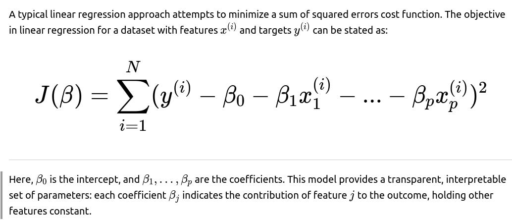
In this case, even if you could train a relatively small neural network or a bigger ensemble model, a simpler linear regression or small decision tree might be the best choice. Linear regression, for instance, will let you quickly see which features (such as marketing spend or historical sales) drive sales forecasts and by how much, while making the reasoning process transparent. Even if a neural network might achieve a slight improvement on the test set, the simplicity and interpretability of a linear regression model could be more critical in ensuring stakeholder trust, avoiding large misallocations of resources, and debugging the model’s predictions.
Why Simpler Models Are Preferred in Safety-Critical and Regulated Environments
In industries such as healthcare, aviation, or autonomous driving, decisions can be life-and-death. Transparency is mandatory for regulatory compliance. A simpler model such as a small decision tree can offer crisp, rule-based decisions that align well with how regulators and domain experts reason about real-world risks. For example, diagnosing a patient with a certain condition might require clear evidence for each step that led to that conclusion. A black-box deep neural network could introduce additional regulatory hurdles, especially if the interpretability methods are not robust or widely accepted.
In many financial applications, a bank might be required to explain loan-approval decisions to potential customers. Relying on a simpler model (or at least an interpretable method) helps ensure legal compliance under rules such as the “Right to Explanation.” Additionally, if the model’s performance in outlier scenarios must be guaranteed, or there are stress-test conditions to meet, simpler models can be easier to verify and stress-test thoroughly.
Key Considerations: Data Size, Overfitting Risk, Interpretability, and Resource Constraints
Data Size and Overfitting Risk If you only have a small dataset, a neural network with millions of parameters can quickly overfit. Simpler models like linear regression or a small decision tree can reduce the risk of overfitting when data is scarce. A smaller hypothesis space often means the model generalizes better with fewer examples.
Interpretability Certain business contexts need easily interpretable models: They facilitate trust with stakeholders, ensuring decisions can be explained. They allow for straightforward identification of which features are most important. They help you quickly debug and refine the model if something goes wrong.
Computational Constraints Neural networks and large ensembles can require powerful GPU clusters or significant memory for both training and inference, which may be impractical in mobile or edge devices. For smaller data sets or real-time predictions in resource-constrained environments, simpler methods are often more effective.
Risk Management in High-Stakes Decisions When a model’s error could lead to huge losses or severe real-world consequences, simpler models might be safer. Auditing or verifying a simpler model’s behavior across different operational settings is often more straightforward.
Mathematical Underpinnings of Model Complexity
By comparison, a deep neural network with multiple layers can approximate highly complex functions. However, the interpretability of each weight is harder to articulate in high dimensions, and explaining how a small change in a certain input affects the final prediction becomes a complex task of analyzing activation layers.
When Simpler Is More Appropriate
Simpler models become a favorable choice in many real-world contexts:
Situations with limited data where overfitting would be a major concern, and a large or deep model might memorize the small dataset rather than generalize. Any regulated industry where model decisions need to be transparent and auditable by humans. Edge computing scenarios, like wearable medical devices, where memory and power constraints severely limit the feasibility of large networks. Fast iteration cycles in startups or small businesses that prioritize easy model updates and require immediate insights into how each predictor influences outcomes. Once your model’s predictions must be explained to non-technical stakeholders, or where legal requirements (like GDPR or compliance rules) demand interpretability.
Implementation Example: Linear Regression in Python
Below is a minimal illustration of how one might train a simple linear regression model using scikit-learn. This is far simpler than building a neural network from scratch or using advanced libraries like PyTorch or TensorFlow. It also trains much faster and remains straightforward to debug and interpret.
import numpy as np
from sklearn.linear_model import LinearRegression

# Suppose X is a 2D numpy array of shape (num_samples, num_features)
# and y is the target array of shape (num_samples,)

# Example dataset (small and easy to interpret)
X = np.array([
    [1.0, 3.2],
    [2.0, 4.1],
    [3.0, 5.5],
    [4.0, 6.7],
])
y = np.array([2.1, 2.9, 3.3, 4.0])

model = LinearRegression()
model.fit(X, y)

# Coefficients and intercept
print("Coefficients:", model.coef_)
print("Intercept:", model.intercept_)

# Making predictions
prediction_example = np.array([])
predicted_value = model.predict(prediction_example)
print("Predicted value:", predicted_value)
From this simple model, each coefficient corresponds to the estimated effect of a feature on the output. We can quickly see how changes in each input dimension affect the final prediction. If the coefficient for the first feature is, say, 0.5, it directly tells you that an increase of 1 unit in that feature is associated with a 0.5 increase in the predicted outcome.
How the Example Demonstrates the Preference for Simpler Models
The code snippet highlights a situation where dataset size is small, and we want immediate clarity on how each feature affects our target. By contrast, a deep neural network might slightly reduce error on a hidden test set but would not necessarily justify the extra complexity. It would also reduce interpretability, which can be critical for high-stakes decisions such as operational planning, manufacturing, or budgeting.
Potential Pitfalls of Choosing Simpler Models
Even though simpler models often solve many problems effectively, one must be aware of possible limitations:
If the underlying relationship is highly non-linear or complex, a linear model might underfit. The resulting errors might be systematically biased, leading to poor performance in certain segments of the data. Some interpretability can be superficial if interaction terms or polynomial transformations are not correctly included when needed. Although linear models are straightforward, incorrectly specified features or omitted relevant variables can lead to misleading results that are “simple” but not accurate.
Despite these pitfalls, in many safety-critical or high-interpretability domains, making a small trade-off in accuracy is worth it to gain clarity, reliability, and stakeholder trust.
What if We Start Seeing Poor Generalization with Our Linear Model?
Sometimes you might worry about poor generalization with your linear regression or small decision tree if the relationship is more complicated. The first step is to look for bias in the residual plots. If there is a distinct structure left in the residuals—like a curved pattern—it indicates the model is systematically missing non-linear behavior. You might consider polynomial terms or introducing mild complexity like ensemble methods. However, even these expansions can be kept at a simpler scope compared to a large neural network, preserving interpretability to a certain degree.
How Do We Know When to Step Up to a Larger Model?
Signs can include consistently poor or biased predictions, especially if it is evident that the phenomenon is highly non-linear (like certain time-series patterns or images). Another major consideration is whether an incremental improvement in accuracy has significant business or safety value. If increasing accuracy by 2% drastically impacts the bottom line or drastically reduces risk, then a more complex model might be justified. You then weigh that gain against your interpretability, computational costs, and regulatory constraints.
Could We Use Hybrid Approaches?
Yes. In many production systems, simpler models are used for day-to-day decisions, while more complex models may be used offline to analyze potential improvements. Or you might use a two-stage approach, where a simple model handles the majority of cases, and only in uncertain or high-risk situations do you resort to a more complex model for a “second opinion.” This balances the strengths of both approaches.
What Are Some Best Practices for Model Validation?
With simpler models, you still apply a rigorous validation strategy:
Perform cross-validation on limited datasets to see if the simpler model is indeed robust or overfitting in some unexpected way. Examine domain-specific metrics such as precision, recall, ROC AUC (if it’s a classification problem), or mean absolute error (if it’s a regression task). Use interpretable metrics like correlation between predictions and ground truth, and analyze partial dependency plots or coefficients to ensure that the model is consistent with known domain expertise.
How to Communicate the Choice of a Simpler Model to Business Stakeholders?
You can highlight several points to non-technical stakeholders:
Explain that the simpler model is faster to train and deploy, so your team can iterate quickly. Reinforce that the simpler model’s transparency is essential for regulatory compliance or for justifying decisions. Demonstrate how the model’s predictions align with domain knowledge, building trust in the model’s correctness. Point out that the data itself might not be sufficient to safely train and generalize a larger, more complex model, which could lead to misleading or risky predictions.
What Are Some Real-World Examples Beyond Business Forecasting?
Medical diagnoses with limited patient data: A small logistic regression or decision tree can be more interpretable for a hospital environment. Insurance risk scoring with strict compliance: Explaining a small decision tree to regulators is often straightforward compared to explaining a complicated black-box model. Predicting machinery failure on a factory floor: If interpretability is required to quickly find root causes of machine faults, a simpler model can be advantageous.
Below are additional follow-up questions
How would you handle concept drift if the simpler model starts to degrade over time due to changes in the data distribution?
Concept drift refers to the phenomenon where the relationship between input features and target outputs changes over time. Even with a simpler model, if the data distribution shifts, the model may fail to generalize as well as it did initially. One effective way to address concept drift is to establish a monitoring pipeline that continuously evaluates model performance on a recent data window. When performance metrics deviate beyond a threshold, you can trigger a partial or full re-training of the simpler model using the newest data.
Another approach is incremental learning, where the model parameters are updated with small batches of fresh data. In linear regression, for example, you can adjust coefficients incrementally without discarding all previous knowledge. However, you must be cautious about catastrophic forgetting, where the model might overfit recent observations and lose the general patterns learned from past data.
Additionally, having domain experts weigh in on whether the new data distribution is truly different from the historical data can be helpful. If external or macro-level factors are driving the shift—such as changes in economic conditions—analysts may incorporate these factors as new features or shift the model’s scope.
In production, you might set up an automated system that checks predictive quality on an ongoing basis (e.g., comparing predictions to ground truth with a daily or weekly lag) and flags anomalies. Smaller, simpler models can be re-trained faster than large, complex models, making them more amenable to frequent updates.
Pitfalls can occur if you re-train too often and introduce noise from transient fluctuations. It is important to track performance stability over multiple time windows to avoid reactionary re-fitting. Another subtlety is that simpler models usually have fewer parameters, so they may adapt to new patterns slower or might require feature engineering that captures changes more explicitly.
Finally, if the simpler model still fails to capture the new relationships even after re-training, you might explore moderate increases in complexity—like polynomial features or piecewise linear models—while still retaining a relative level of interpretability. The key is balancing the risk of underfitting the new distribution against the need to retain interpretability and ease of updating.
What if there’s a significant difference in the costs of false positives vs. false negatives—how would that influence the choice of a simpler model?
When false positives and false negatives have disproportionate impacts, it is crucial to tailor the model's decision boundary and threshold in a way that addresses these asymmetric costs. Even with a simpler model—like logistic regression or a small decision tree—you can weight instances differently in the loss function or adjust decision thresholds post-training.
In logistic regression, for instance, you might incorporate class weights to penalize misclassifications of the minority or more costly class more severely. This can help the model focus on the type of errors that carry higher real-world consequences. Alternatively, once the model is trained, you can shift the decision threshold (e.g., from 0.5 to a higher or lower cutoff for positive classification) to prioritize one error type over the other.
In domains like fraud detection, a false negative (missing an actual fraud) can be very costly, so you would want to calibrate the threshold to minimize those missed cases. With a simpler model, the process of adjusting or explaining threshold moves is transparent: you can demonstrate how shifting a threshold affects metrics like precision, recall, and the confusion matrix.
A potential pitfall arises if the underlying data distribution is highly imbalanced. A simpler model might struggle to capture rare classes or complex boundary regions. Careful sampling strategies—like oversampling the minority class or undersampling the majority—are often needed. Another pitfall is that naive weighting strategies might cause overfitting, especially if the dataset is small. Validating these weighted or threshold-tuned approaches with cross-validation helps confirm their reliability.
Ultimately, the choice to remain with a simpler model must be evaluated alongside these cost considerations. If the cost disparity is extremely large and requires modeling subtle feature interactions, a more sophisticated approach might yield better cost-adjusted performance. However, you can often strike a balance using a simpler model, especially if domain experts can guide the weighting and threshold strategies accurately.
How do you perform robust feature engineering to ensure a simpler model captures the necessary relationships in the data?
In simpler models, feature engineering can play an outsized role in capturing the underlying relationships that the model alone cannot approximate with its limited complexity. For a linear model, transformations like polynomial terms (e.g., squaring or interaction terms between key features) can allow the model to handle mild non-linear effects without entirely sacrificing interpretability.
Domain knowledge is critical. For instance, if you know that a certain ratio of two variables (e.g., “marketing_spend / number_of_website_visits”) is highly predictive, you can directly create a feature for that ratio. Simpler models often benefit significantly from these domain-driven transformations.
You might also incorporate feature scaling methods such as standardization (subtract mean, divide by standard deviation) to help linear regression converge more efficiently and treat all features more equitably. Decision trees are typically more robust to varying scales, but they can still benefit from meaningful feature construction, such as time-based features in a seasonality context.
A potential pitfall is inadvertently introducing too many engineered features, leading the simpler model to overfit. Regularization techniques like or can provide a safeguard by shrinking coefficients of less important features. Another subtle risk is introducing correlated features that make model interpretation more challenging; a domain expert might be confused if multiple features effectively encode the same phenomenon in different ways.
Robust validation is essential to confirm the added feature indeed improves performance in a generalizable way. Techniques like cross-validation and out-of-time validation (especially for time-series data) are recommended to test the real impact of newly engineered features. By carefully combining domain insight with systematic experimentation, you ensure that your simpler model has enough expressive power without becoming a black box.
In which ways might you incorporate domain knowledge into simpler models to enhance interpretability and performance?
Domain knowledge can shape the entire modeling strategy. A few common ways to embed domain insights include selecting features that are known causal drivers, creating composite features that reflect domain-specific interactions, and applying constraints or priors that align with expert understanding. For example, in a medical context, you might encode known symptom combinations or risk factors as separate binary features.
For a linear regression model, domain experts could specify sign constraints on coefficients if it is known that a relationship must be positive or negative. This ensures the model's behavior aligns with established theory. Decision trees can incorporate domain rules as initial splitting constraints or pre-processing steps that reduce the search space.
In heavily regulated environments, you might consult domain experts and regulators to co-design a maximum allowable depth for decision trees or to limit the set of features to only those that pass legal compliance checks. This might sacrifice some predictive power but ensures the model remains transparent and acceptable to regulatory bodies.
A subtle edge case arises when domain knowledge conflicts with the data-driven patterns. For instance, the data might show an unexpected correlation that domain experts cannot explain. Balancing trust in domain expertise with empirical evidence is tricky: sometimes domain experts revise their hypotheses, while other times you discover data quality issues.
The key advantage of simpler models is that they make it easier to merge domain knowledge with data insights. You can iteratively refine features, apply constraints, and check if the model’s coefficients or splits align with domain rationale. This synergy can yield a model that not only performs robustly but can also be confidently explained to stakeholders.
How do simpler models handle high-dimensional data, and what pitfalls can arise in this scenario?
High-dimensional data means you have a large number of features compared to the number of observations. Linear models can face a severe risk of overfitting if regularization is not used. Applying regularization (Lasso) can help by forcing many coefficients to zero, thus performing feature selection automatically. Alternatively, regularization (Ridge) shrinks coefficients, helping control variance.
Small decision trees can quickly overfit in high-dimensional spaces because they may find very specific splits that appear predictive in training but fail to generalize. Limiting tree depth, pruning, or using something like a single-level decision stump might be necessary to avoid memorizing spurious correlations.
One pitfall is that in very high dimensions, interpretability can still suffer, even if the model is linear—there might be hundreds of non-zero coefficients. Stakeholders might not realistically parse all those coefficients or how they interact, undermining the simplicity advantage.
Another subtlety is the curse of dimensionality: you might not have enough data points to reliably estimate the contribution of each feature, resulting in unstable coefficients. Cross-validation becomes critical to detect overfitting. If your main reason for choosing a simpler model is interpretability, you might further reduce dimensionality (e.g., via domain-driven feature selection or unsupervised methods like PCA) before fitting. However, PCA-based transformations can hamper direct interpretability because the new features become linear combinations of the original ones.
In practice, a balance of manual feature selection, domain knowledge, and regularization strategies can help simpler models remain robust in high-dimensional settings. But if performance remains poor, it might signal that a more complex model (e.g., with carefully designed embeddings) could be required.
Can simpler models be beneficial when the data has strong temporal dependencies, such as in time-series analysis? Under what conditions might they fail?
Simpler models can indeed be useful in time-series contexts, particularly if you have well-known seasonal patterns or a strong trend that can be captured by a small set of features (e.g., lag features, moving averages, or seasonal indicators). For instance, an ARIMA model or a linear regression with lagged target variables could be sufficient if the time-series is relatively stable and linear in its dynamics.
They might fail if the time-series is highly non-linear or exhibits regime shifts. For example, if consumer behavior changes drastically following an external event, a purely linear model might not capture the sudden transition. Similarly, if there are interactions between multiple seasonality factors (daily, weekly, yearly), simpler models may struggle unless you explicitly engineer features for each seasonality type.
Another scenario where simpler models can fail is if the time-series includes complicated external variables (holidays, promotions, macroeconomic shocks). In principle, you can incorporate them into a simpler model, but if the interactions are too intricate, you risk either oversimplifying or building an excessively large set of derived features.
A subtle pitfall is ignoring autocorrelation in the residuals. If you try using a vanilla linear regression without addressing temporal correlation, standard errors and significance tests for coefficients can become unreliable. In these situations, specialized time-series regression models or hierarchical models with fewer assumptions might be safer options.
That said, simpler models are often easier to maintain and re-train in a rolling or expanding window scenario, which is common in time-series forecasting. Frequent re-training helps adapt to new data and changing trends. If the domain environment is stable and changes are relatively predictable, simpler time-series models are an excellent choice for clarity and reliability.
How do you approach model calibration and uncertainty quantification in simpler models?
Model calibration ensures that predicted probabilities (or predictions) align well with observed outcomes. With logistic regression, calibration is typically straightforward because outputs can be interpreted as probabilities, especially if you have sufficient data. Calibration plots can confirm whether the probabilities need adjustment. If miscalibration is present, techniques like isotonic regression or Platt scaling can be applied.
For regression tasks, you might quantify uncertainty by constructing prediction intervals. With linear regression, you can derive confidence intervals around the predictions based on the variance estimate of the residuals. However, these assumptions rely on the residuals being approximately normally distributed and homoscedastic. Real-world data can violate these assumptions, so you may need robust standard error estimators or non-parametric methods like bootstrapping to capture the true uncertainty.
A subtle point arises if the data distribution is highly skewed or if outliers are present. Outliers can inflate variance estimates, leading to overly wide intervals. Robust regression techniques (e.g., using M-estimators) can mitigate this.
Another pitfall is ignoring potential correlation among features, which might invalidate naive confidence interval assumptions. Even in simpler models, carefully diagnosing residual plots and checking for correlation patterns is essential.
Overall, simpler models make it easier to explain how these intervals and calibration adjustments are derived. Business stakeholders or regulators may feel more comfortable trusting a linear model’s interval estimates than the more opaque methods used to approximate uncertainty in deep neural networks.
What are typical infrastructure and deployment considerations when you choose a simpler model for large-scale inference?
When deploying a simpler model at scale, the computational and memory footprint is typically smaller, making it easier to serve predictions in real-time. A linear model might only need to store a few thousand coefficients in memory, which can be done even on constrained hardware.
Batch scoring can also be handled efficiently, because matrix multiplication with a coefficient vector is straightforward to optimize. Frameworks like scikit-learn or even lightweight libraries in C++ or Java can be used to serve the model with minimal latency. If you have billions of instances to score, simpler models can be parallelized easily across a cluster.
A potential edge case arises when your feature engineering pipeline is complex. Even if the model itself is simple, you might incur substantial overhead in transforming raw input into the final feature set. Ensuring your feature pipelines are consistent between training and inference environments is critical.
Monitoring is simpler, too. If you see a sudden drift in predictions, you can quickly trace it back to changes in a particular coefficient or a shift in certain input values. In larger models, the debugging process might require advanced observability tools.
Another subtlety is version control. As you update coefficients or transform logic in simpler models, it’s easy to keep track of changes using standard deployment workflows. Larger models may require artifact management for multi-gigabyte model checkpoints. For businesses prioritizing reliability and minimal overhead, simpler models can drastically reduce dev-ops complexity without sacrificing too much performance.
How can you incorporate fairness or bias mitigation strategies more easily in simpler models, and what pitfalls remain in regulated domains?
Fairness and bias mitigation often involve interventions like removing sensitive attributes (e.g., gender or race), re-weighting instances, or adjusting decisions post-hoc. With a simpler model, such strategies are often more transparent and easier to control. For example, in a linear model, you can explicitly check the coefficient for sensitive features or correlated proxies and set constraints or adjust how these features enter the model.
One approach might be to use separate intercept terms for different protected groups (sometimes called “group-wise calibration”) to ensure the model does not systematically favor one group over another. You can also examine partial dependence plots for protected attributes in a small decision tree to see how the splits might create disadvantages.
However, a major pitfall is that simply removing protected attributes may not remove bias if other features act as proxies (for instance, ZIP code might strongly correlate with race in some regions). While it’s easier to identify and remove correlated features in a simpler model, you still need deep domain knowledge to avoid inadvertently perpetuating unfairness.
In regulated domains, you must also document each step in the fairness pipeline. Simpler models make it more straightforward to produce the documentation regulators require, such as explaining how each feature influences decisions. Nonetheless, fairness metrics can be multi-faceted—there’s no one-size-fits-all solution. A model can be fair on one measure (e.g., demographic parity) but unfair on another (e.g., equalized odds). Balancing these metrics is a continuous process that typically involves stakeholder input, especially in high-stakes applications like lending, hiring, or medical diagnoses.
How do you approach ensemble methods that combine multiple simpler models, and are they still considered “simple” or do they lose interpretability?
Ensembling multiple simpler models—such as bagging small decision trees (Random Forest) or blending multiple linear models—can often boost performance without resorting to a massive neural network. While each base model is individually simpler, the ensemble’s overall complexity can increase significantly, especially if it consists of dozens or hundreds of components.
For instance, a Random Forest is conceptually a collection of independent decision trees, each trained on a bootstrap sample of the dataset. The final prediction is typically the average (for regression) or majority vote (for classification) across trees. While each individual tree might be shallow, the ensemble can exhibit highly non-linear decision boundaries. This can lead to strong performance but significantly reduces interpretability.
Some interpretability can be regained by examining aggregate statistics (like feature importance measures) or analyzing the distribution of predictions across all trees for a given input. However, you lose the straightforward “if-then” paths that a single small decision tree provides.
A subtle pitfall is that if your main reason for sticking with simpler models is direct interpretability (or regulatory constraints), ensembles can undermine that objective even if each component is simple in isolation. You should clarify whether your stakeholders require local interpretability (how a single prediction is made) or global interpretability (understanding the entire model’s logic).
Ensembles can also be more resource-intensive in inference, especially if you have many components. On the other hand, they are still typically lighter than large deep networks and can often be parallelized. Ultimately, the choice to ensemble simpler models depends on whether you value the trade-off of improved accuracy versus partial loss of interpretability. If you need a small bump in performance while maintaining moderate transparency, a small ensemble (e.g., an average of two or three simple models) might suffice.