
ML Interview Q Series: Would applying a square root to a classifier’s scores alter the ROC curve, and what transformations would?
📚 Browse the full ML Interview series here.
Short Compact solution
Because the ROC curve depends only on the relative ordering of predicted scores (i.e., it is invariant to any strictly increasing transformation), taking the square root does not change the ROC curve. If one score is larger than another, its square root remains larger. As a result, the set of true positive rates and false positive rates at all thresholds remains identical. On the other hand, any function that disrupts the ordering of the scores (for example, a non-monotonic function such as

Comprehensive Explanation
Overview of ROC Curves and Score Transformations
The ROC (Receiver Operating Characteristic) curve is constructed by plotting the true positive rate (TPR) against the false positive rate (FPR) at various threshold levels. A “score” for each instance—here, a probability estimate that the instance is positive (fraudulent)—is thresholded to decide whether an instance is classified as positive or negative. By varying that threshold from 0 to 1, you trace out a curve representing the trade-off between TPR and FPR.
A key insight is that the shape of an ROC curve depends entirely on the rank ordering of the scores rather than their absolute values. Specifically:
If score A is higher than score B in the original scale, and you apply a transformation that is strictly monotonically increasing (e.g., square root, exponential, linear scaling with a positive slope, etc.), A will remain higher than B in the transformed scale.
Since the thresholds used to construct the ROC curve will shift accordingly, the positions of the points on the TPR/FPR curve do not change; hence the ROC curve itself remains identical.
Why Square Root Preserves Ordering

. Because of this monotonic relationship, the relative order of all scores from different loan applications remains unaltered when you take the square root of each score. Consequently, at every possible threshold level, each instance’s classification (as positive or negative) remains the same as in the original scale. The TPR and FPR values at each threshold remain unchanged, so the ROC curve is not affected.
Examples of Functions That DO Change the ROC Curve

If you take a score and negate it, higher scores become lower in the transformed scale. An instance with a higher probability would end up having a lower post-transformation value than one with a slightly lower probability—this reverses the ordering.

(and in fact reverses the order for values above 0).
Stepwise or Non-Continuous Jumps: A piecewise function that groups different input values into the same output intervals can cause multiple distinct scores to collapse to the same level, losing the finer ordering structure.

Any transformation that is not monotonic (or at least not consistently increasing over the domain) risks reordering at least some of the scores. Reordering leads to different TPR and FPR patterns, thus different points in the ROC space and a different ROC curve.
Threshold Shifts vs. Score Reordering
One important note is that applying a strictly increasing transformation will typically shift the exact numeric thresholds you use to separate classes, but it will not affect the TPR/FPR pairs or the area under the ROC curve (AUC). The classification boundaries in terms of the original probabilities may look different after transformation, but the ranking of the data points stays the same. That is the pivotal reason why such a transformation has no impact on the ROC curve.
What follows are several deeper follow-up questions and thorough answers:
How does monotonicity ensure the ordering remains the same?
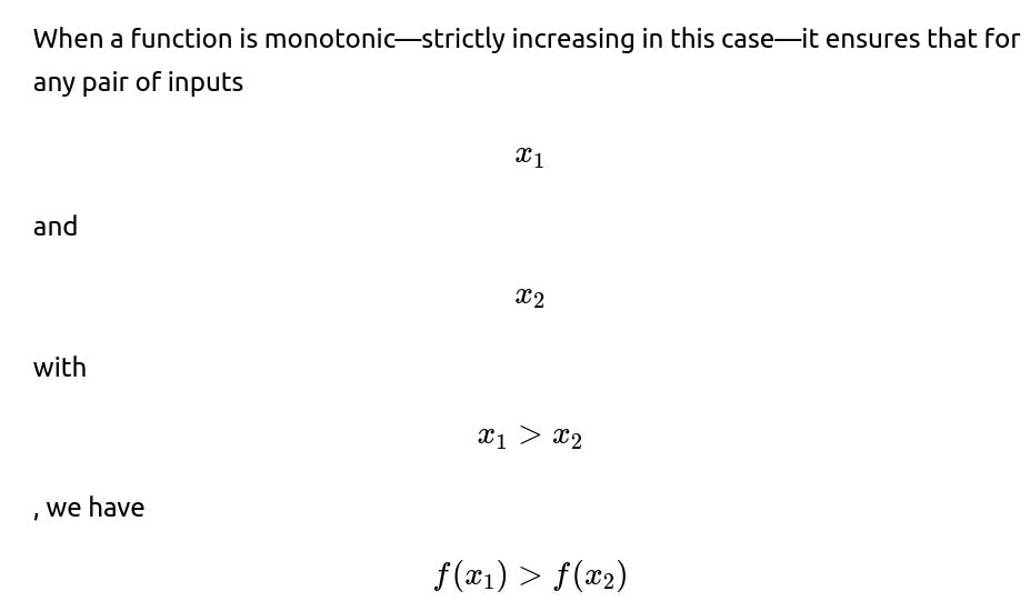
. No matter how many scores you have, their order relative to each other is preserved. Since ROC curves rely on sorting the scores from highest to lowest (or vice versa) to determine how classification thresholds move from labeling nearly all instances negative to labeling them all positive, a strictly increasing function does not alter that rank.
What happens if the function is only weakly increasing or piecewise constant?
If the function is not strictly increasing but is non-decreasing overall, you might end up with ties where some distinct scores map to the same transformed value. This can cause partial changes in the distribution of scores, potentially causing slight alterations in how thresholds are applied. Usually, if it’s purely non-decreasing (even if some values get mapped to the same number), the ordering (except for tied points) is mostly intact. Thus, in many practical cases, a merely non-decreasing function still yields the same or a very similar ROC curve. However, stepwise or “piecewise constant” mappings can lead to many ties and the final shape might shift if the number and positions of unique threshold values become significantly different.
Can applying the square root to scores below 1 cause any practical numerical issues?
In principle, there are no conceptual issues with taking the square root of values in [0,1]. Numerically, though, for extremely small probabilities (close to 0), the square root will shift them higher on an absolute scale (e.g., 0.0001 becomes 0.01), while still keeping them less than any value greater than 0.01. The relative ranking remains the same, so there is no problem for the ROC curve. In extremely edge case scenarios, floating-point precision might come into play if many scores are extremely small, but for typical double-precision floats used in frameworks like TensorFlow or PyTorch, this usually isn’t problematic.
Does this also mean the Area Under the Curve (AUC) remains the same?
Yes. The AUC metric is equivalent to the probability that a randomly chosen positive sample has a higher score than a randomly chosen negative sample. Since monotonic transformations do not alter the probability ordering of scores for positive vs. negative samples, the AUC is unchanged.
Could you show an example of how to verify this practically?
You could write a short Python script that generates two sets of simulated scores: one set for positives, one for negatives. Calculate the AUC on the original scores, then apply a strictly increasing function (like square root). Recompute the AUC. You’ll see the AUC remains the same.
import numpy as np
from sklearn.metrics import roc_auc_score

# Suppose we have some synthetic scores
np.random.seed(42)
pos_scores = np.random.rand(1000) * 0.8 + 0.2  # Simulate positive scores
neg_scores = np.random.rand(1000) * 0.5       # Simulate negative scores

# Create labels
labels = np.array([1]*1000 + [0]*1000)

# Combine scores
all_scores = np.concatenate((pos_scores, neg_scores))

# Compute AUC before transformation
auc_before = roc_auc_score(labels, all_scores)

# Apply square root
transformed_scores = np.sqrt(all_scores)

# Compute AUC after transformation
auc_after = roc_auc_score(labels, transformed_scores)

print("AUC before transformation:", auc_before)
print("AUC after transformation :", auc_after)
You would find that “AUC before transformation” and “AUC after transformation” are extremely close (often exactly the same to within floating-point tolerances).
Why do non-monotonic functions break the ROC invariance?
When a transformation can map higher original scores to lower transformed scores (or vice versa), the rank ordering changes. A previously less likely instance could end up having a higher transformed score than a previously more likely instance. This reordering changes the TPR-FPR progression as thresholds move, thus altering the shape of the ROC curve and typically the AUC as well.
What if we only care about a specific threshold, not the entire ROC?
If you fix a single threshold of interest and apply a strictly increasing transformation, the numeric threshold in the new space will be different, but you can still find an equivalent threshold to recover the same classification. So for a single threshold, as long as the function is strictly increasing, you can always “rescale” the threshold to maintain the same classification decisions. Therefore, the outcome at that specific threshold remains the same.
If your function was non-monotonic, you cannot simply adjust a single threshold to reproduce the same classification decisions in all cases because multiple original scores might map inconsistently to the new scale.
Summary of Key Takeaways
ROC curve depends solely on the ordering of the scores when varying thresholds from 0 to 1.
Monotonically increasing transformations (like square root) do not alter score ordering, so the ROC curve remains the same.
Non-monotonic transformations can reorder scores, leading to changes in TPR and FPR across thresholds, thus modifying the ROC curve.
AUC remains invariant under any strictly increasing mapping since AUC also relies only on the rank ordering of positive vs. negative scores.
Below are additional follow-up questions
Does monotonic transformation preserve other metrics beyond the ROC curve, such as Precision-Recall curves?
Precision-Recall (PR) curves reflect the relationship between precision (the fraction of predicted positives that are truly positive) and recall (the fraction of total positives that are correctly predicted) across different classification thresholds. Although the ROC curve and the PR curve both rely on ranking of scores to some extent, the behaviors of these two curves can differ because precision depends heavily on the proportion of positive predictions relative to total predictions.
A strictly increasing transformation still preserves the ranking, so the relative order for “most likely positive” to “least likely positive” remains unchanged. At each threshold level, you end up classifying the same set of instances as “positive.” Thus, the recall (TP / (TP + FN)) and the precision (TP / (TP + FP)) at each threshold end up being the same, which means the Precision-Recall curve should also remain the same in an idealized scenario. In practice, numerical tie situations—if the transformation is merely non-decreasing—could slightly alter how the threshold picks positives vs. negatives.
A subtle pitfall can emerge if multiple score values are clustered around 0 or 1 and the transformation causes small numeric differences to collapse (e.g., if the transformation is piecewise constant in some region). Then some previously distinct scores might map to the same transformed value. In such a scenario, you could cause shifts in how thresholds sort or group certain samples, potentially altering the precision-recall curve slightly. But if your transformation is strictly and smoothly increasing across the entire [0,1] domain, then PR curves remain structurally the same, just as ROC curves do.
How does data distribution interact with monotonic transformations in real-world scenarios?
In many real-world applications, predicted scores can cluster at specific ranges. For instance, a classifier might assign most negatives around 0.0–0.1 and most positives around 0.9–1.0. In such heavily skewed distributions, applying a monotonic transformation like the square root might still preserve ordering overall, but the range in which most scores fall could become more compressed or expanded.
For example, if a huge fraction of negative samples initially have very small scores near 0, then taking the square root of those small values will push many negatives to relatively higher numbers compared to their original values. This might raise concerns about interpretability or about how thresholds in the new scale reflect the actual probabilities.
However, from a pure ranking perspective—and thus from the standpoint of the ROC curve—this distortion does not matter: the instance that used to have a higher score than another is still higher after the transformation. In production, though, your business or application might interpret these “shifted” values differently, leading to confusion if stakeholders are used to the original numeric range. So a key subtlety is that the ROC curve’s shape remains the same, but your team might have to adjust how it interprets and sets thresholds in a way that’s consistent with the new distribution.
Could partial transformations (i.e., transformations that only apply to certain score intervals) preserve the ROC curve?
In principle, partial transformations can preserve the ordering of scores within those intervals and could keep the same global ranking if each sub-range transformation remains strictly increasing and the boundaries between intervals align in a way that preserves the overall order. However, this is trickier to execute correctly. For example:

If the boundary value at 0.5 is mapped to a new value that falls outside the correct ordering relative to values just below or above 0.5, you could easily break the global monotonic order.
Hence, a partial transformation can still maintain the overall ranking only if you ensure that each piece is strictly monotonic and all pieces align smoothly at their boundaries. Otherwise, you create a “kink” that can reorder some values across the boundary. This is an important edge case because developers or data scientists might attempt custom calibrations or binning for certain score ranges without noticing that they invert or overlap boundaries, which would change the final ROC.
When does a strictly monotonic transformation become problematic for practical calibration, even though the ROC curve remains intact?
Calibration is about ensuring that predicted probabilities align well with real-world frequencies. For example, if a model predicts a probability of 0.7 for a sample, we ideally want about 70% of the samples with that predicted probability to be truly positive. Monotonic transformations can alter the interpretation of these probabilities:
Even though the ROC curve remains the same (since the ranking of scores is unchanged), the new scores may no longer represent well-calibrated probabilities. A square root transform of a probability that was originally 0.9, for instance, becomes about 0.95, which suggests a higher probability of being positive, even though from the model’s perspective there is no actual difference in rank.
In certain domains, you might require well-calibrated outputs for downstream tasks (e.g., risk assessments in finance). A purely monotonic but arbitrary transformation could destroy calibration while leaving the ROC unaffected.
This is a subtle pitfall because some practitioners might believe that if ROC is unchanged, then the overall “model performance” is fine. In reality, if you need well-calibrated probabilities, you might have to perform an additional calibration procedure (e.g., Platt scaling or isotonic regression) rather than just rely on the unadjusted transformed outputs.
Could the use of floating-point precision or numeric stability affect ranking after monotonic transformations?
Yes. In high-dimensional or large-scale applications, numeric stability can become a hidden pitfall. Consider:
If two scores are extremely close in floating-point representation, applying a transformation with limited floating-point precision might map them to the same value or slightly reorder them. This effect can show up in GPUs using lower-precision data types (like float16) or in large-scale inference with mixed precision.
Although such changes in order might only affect a tiny fraction of samples, if your data is extremely large or your threshold is near a critical range, these small changes could have an observable effect on your final classification performance or cause minor fluctuations in the ROC curve. Usually, the difference might be negligible, but in very sensitive domains—like medical diagnosis—it’s important to verify your numeric assumptions.
Therefore, in practice, you have to be aware of how close your numeric values are and whether your transformation can cause collisions or near-collisions in floating-point space.
How do monotonic transformations interact with ensemble methods that average scores from multiple models?
Ensemble methods often combine the outputs of multiple models, sometimes by averaging their predicted probabilities. If each individual model’s score is in [0,1], the final ensemble score is also typically in [0,1]. Now, imagine you apply a monotonic transformation to each individual model’s score before averaging. In that case:
Within each model, the ordering of that model’s predictions is preserved, but once you combine them (e.g., by a simple arithmetic mean), the final ordering might change relative to the original averaged scores.
This is because the mean of transformed values does not necessarily preserve the original rank ordering that you would have gotten by first averaging the raw probabilities and then transforming. In other words, “transform-then-average” can differ from “average-then-transform,” and these two procedures can produce different final rank orders for some instances.
A pitfall emerges when you assume that because each individual model’s transformation is monotonic, the final ensemble ordering is also guaranteed to remain the same. It is not, unless you transform the final combined score, which would maintain overall ordering. But if you transform each model’s score separately and then aggregate, you effectively create a new scoring function that is no longer a simple monotonic transformation of the original average.
Hence, to preserve the same ordering in an ensemble scenario, you want to apply transformations on the combined (averaged or otherwise aggregated) score, not on each model’s output before combination.
Are there domain cases where the notion of “monotonic” might be ambiguous?
Sometimes, probabilities or risk scores are only valid over a specific data segment, and outside that segment, the model might produce special outputs (like “N/A” or a sentinel value). If a post-processing routine is designed to map sentinel values to a fixed number, you could inadvertently reorder that sample relative to legitimate scores. For instance, you might produce an “impossible” negative score for an out-of-distribution sample, or set it to a default 0.5. This could break the assumption that the transformation is truly monotonic across the entire domain used by the scoring engine.
Another scenario is if the model outputs a custom type that is not purely numeric (e.g., certain rule-based or linguistic confidence measures). Then you attempt to force a numeric transformation that might treat some “unknown” category in an ad hoc way. Ensuring monotonicity becomes non-trivial if your domain includes these special categories or discontinuities.
How might post-processing transformations affect decision curve analysis or cost-sensitive evaluations?
Beyond ROC and PR analysis, practitioners sometimes use decision curve analysis or cost-sensitive evaluations. Decision curve analysis weighs the clinical or business implications of certain threshold choices. For instance, in a finance context, you might have a varying cost of false positives vs. false negatives. While a strictly increasing transformation will keep the rank-based results identical, the relationship between the raw probability estimates and the actual cost model might shift. For example:
If your threshold is chosen based on expected cost or utility, you may rely on probabilities to estimate the expected losses or gains. Transforming the scores might require you to recalibrate your cost function to maintain the same operational threshold.
A pitfall is failing to recalculate the cost threshold in the new transformed scale, which could lead to suboptimal decisions even though the rank ordering is preserved.
Thus, while the ROC remains unchanged, the direct mapping to real-world decisions might need re-tuning to ensure consistent outcomes.
What if the monotonic transformation is applied in a scenario where some scores are originally above 1 or below 0?
Realistically, a model’s raw “probability” output might not always lie strictly within [0,1]—certain algorithmic outputs or uncalibrated logits can be in ranges extending outside [0,1]. For instance, logistic regression sometimes yields numeric instability or partial scoring that, due to rounding or design, goes slightly above 1 or slightly below 0. If you forcibly apply the square root or another function that expects nonnegative inputs, you need to clamp or adjust those out-of-bound values. That clamp can reorder the boundary points if you aren’t careful.
For instance, if a model erroneously outputs 1.02 for one sample and 0.99 for another, and you clamp anything over 1.0 back to 1.0, you’ve now made those two scores identical in the transformed space, even though originally 1.02 was higher than 0.99. In principle, that might not drastically affect the ROC curve if the number of such out-of-range scores is negligible. But in edge cases, especially if many scores end up clamped, the resulting ties can modify the thresholds at which TPR and FPR shift. Therefore, a safe approach is to correct or calibrate scores so they remain in a valid domain prior to transformation, preserving consistent ordering in the process.
How do we ensure interpretability if the ROC curve remains the same but the numeric scale changes drastically?
In many production or stakeholder-facing settings, interpretability and clarity of the model’s outputs are as crucial as performance metrics. If you apply a transformation like the square root or any other strictly increasing function, your ROC curve doesn’t change, so you haven’t lost rank-based performance. Yet the actual numeric values might be very different from the original probabilities.
A manager or clinician might ask why a particular user is flagged with a risk score of 0.8 after transformation, whereas previously that same user had 0.6. Explaining that both represent the same rank is crucial.
Proper documentation of the post-processing transformation is necessary to ensure that any domain experts reading the scores understand that the new “probabilities” are not truly calibrated in the conventional sense. They are effectively a re-mapping that preserves ordering for classification metrics.
This highlight shows the real-world pitfall: teams must ensure that any numeric outputs provided to end-users or domain experts are either left in a calibrated probability space or are clearly labeled as “scores” with no direct interpretation as probabilities.