ML Interview Q Series: Z-test or t-test: Hypothesis Testing with Known vs. Unknown Population Variance.

Browse all the Probability Interview Questions here.
How would you define a Z-test, and under which circumstances would you prefer it over a t-test?
Short Compact solution
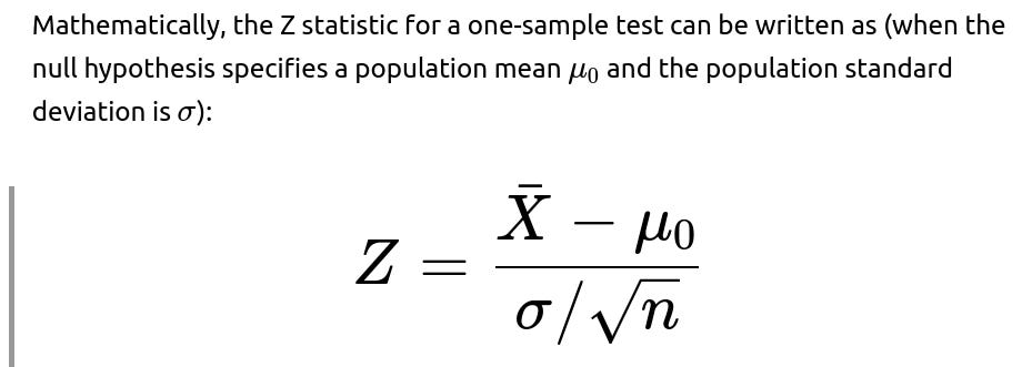
In a Z-test, the test statistic is assumed to follow a standard normal distribution if the null hypothesis holds. In contrast, a t-test uses the Student’s t-distribution under the null. If we are testing the population mean, we can use either a Z-test or a t-test when the distribution of the sample mean is normal or approximately normal (for instance, if the original population is normal or if the sample size is large, such as at least 30, via the Central Limit Theorem).
If the population standard deviation is known, we typically use a Z-test; if it is unknown and must be estimated from the sample, we use a t-test. For very large samples (often above 200), the t-distribution approaches the normal distribution so closely that a Z-test and a t-test produce nearly the same results.

Comprehensive Explanation
Key Distinction Between Z-test and t-test
A Z-test is used when:
Population Standard Deviation is known (or one can assume precise knowledge of it).
The sample size is sufficiently large or the distribution is inherently normal, making the sampling distribution of the mean approach normal.

A t-test is used when:
The population standard deviation is not known and must be estimated from the sample data.
The sample size can be smaller; the t-distribution incorporates uncertainty from estimating σ.
For a one-sample t-test, the test statistic is:

where S is the sample standard deviation, which estimates the unknown σ. Because we are using an estimate for σ, the t-distribution is more spread out (has heavier tails) than the standard normal distribution, especially for smaller sample sizes. Its shape is determined by the degrees of freedom, usually n−1 for a one-sample t-test.
Normality Requirements
Both tests usually assume that the sample mean is drawn from a distribution that is normal or that the sample size is large enough for the Central Limit Theorem to hold. If n≥30, many practitioners rely on the Central Limit Theorem, making the mean approximately normally distributed even if the original population is not perfectly normal.
If the population is known to be heavily skewed or has strong outliers, more robust methods might be considered, or one might apply transformations or use non-parametric tests (like Wilcoxon signed-rank) if normality is seriously violated.


Large Sample Sizes and Convergence of t to Z
When the sample size n grows large (some say n>200, others might pick n>30 or n>50 depending on context), the t-distribution converges to the normal distribution. Thus, with large samples, the difference between a t-test and a Z-test is minimal.
Practical Considerations
Confidence in Knowing σ: In real situations, truly knowing the population standard deviation is somewhat rare (unless it’s a well-studied phenomenon). If you are uncertain about σ, it is generally safer to assume it’s unknown and use a t-test or some alternative approach.
Sample Size: If n is small (say less than 30) and σσ is unknown, the t-test is the more appropriate choice, provided that the underlying population is roughly normal.
Robustness to Outliers: Outliers can inflate the sample standard deviation S, which can reduce the power of the t-test. Strategies such as outlier handling, data transformations, or adopting non-parametric tests might be considered, depending on the scenario.
One-sided vs Two-sided: Both Z-tests and t-tests can be formulated as one-sided or two-sided. The choice depends on the hypothesis being tested.
What if the Sample Size is below 30?
If the population standard deviation σ is unknown and the sample size is quite small (less than 30), the t-test is generally recommended, assuming the population distribution is reasonably normal. The t-distribution will correctly account for the extra uncertainty from estimating σ with so few observations.
What if the Underlying Distribution is not Normal?
If the sample size is small and the data distribution is significantly non-normal, the t-test might not be valid. One can consider:
Using non-parametric alternatives such as the Wilcoxon signed-rank test (for a one-sample or paired design) or the Mann–Whitney U test (for two independent samples).
Applying data transformations to make the distribution closer to normal.
Could We Ever Use a Z-test When the Population Standard Deviation is Unknown?
In some real-world analyses, if the sample size is extremely large, you might approximate the population standard deviation with a very precise sample standard deviation. Many practitioners then treat it “as if” it is known and use a Z-test. Strictly speaking, it’s more correct to use a t-test, but for very large n, the difference is negligible.

Handling a Two-Sample Test Scenario
For comparing two means:
Two-sample Z-test: used if both population standard deviations are known and the distributions are normal or the sample sizes are large.
Two-sample t-test: used more commonly when neither population’s standard deviation is known. If you assume equal variances, you pool the variance; otherwise, you use a Welch’s correction for unequal variances.
Does the Test Differ if It Is One-tailed or Two-tailed?
The fundamental formula for the test statistic remains the same (Z or t). However, for one-tailed tests, the rejection region is only on one side of the distribution. For two-tailed tests, the rejection region is split across both tails. Conceptually, you choose a one-tailed test only if the research question genuinely concerns a specific direction of effect (e.g., testing if a mean is greater than some value vs. simply different from that value).
Potential Pitfalls
Misinterpretation of p-values: Always remember the assumptions under which the p-value is valid, especially normality and independence of observations.
Multiple Testing: If running multiple t-tests, you might need to correct for multiple comparisons to control the overall Type I error rate.
Small Sample, Unknown Variance: Using a Z-test blindly when n is tiny and σ is unknown can lead to invalid or misleading results.
Additional Follow-up Questions
How Would You Conduct These Tests in Python?
You can use libraries like SciPy for t-tests. For example:
import numpy as np
from scipy import stats

# Example data
sample_data = np.array([2.5, 2.8, 3.0, 2.4, 2.9])

# One-sample t-test against hypothesized mean mu=2.7
t_stat, p_value = stats.ttest_1samp(sample_data, 2.7)
print("t-statistic =", t_stat, "p-value =", p_value)
For a Z-test, Python’s standard libraries do not have a built-in function because it’s less commonly used in practice. However, you can implement it manually if you know σ:
import numpy as np
import math
from scipy.stats import norm

# Known population std
sigma = 0.5
mu_0 = 2.7
sample_data = np.array([2.5, 2.8, 3.0, 2.4, 2.9])

sample_mean = np.mean(sample_data)
n = len(sample_data)

z_stat = (sample_mean - mu_0) / (sigma / math.sqrt(n))
p_value = 2 * (1 - norm.cdf(abs(z_stat)))  # two-sided p-value
print("Z-statistic =", z_stat, "p-value =", p_value)
Can You Use a Paired t-test in This Context?
A paired t-test is used when you have paired observations (e.g., before-and-after measurements on the same subjects). The key difference is that you compute the differences within each pair and perform a one-sample t-test on those differences. It still uses the t distribution but focuses on the paired differences rather than two independent groups.
How Do You Interpret Confidence Intervals in a Z-test vs a t-test?

If a Test is Statistically Significant, Is It Always Practically Important?
Not necessarily. Statistical significance means the observed difference is unlikely to be due to random chance, assuming the null hypothesis is true. Practical significance (or effect size) addresses how large the difference is in real-world terms. It is possible to achieve statistical significance with very large sample sizes, even for a tiny effect that is not meaningful in practice. Therefore, always consider effect sizes (e.g., Cohen’s d, difference of means, or confidence intervals) alongside p-values.
How Do You Check if the Sample is Large Enough to Use the Central Limit Theorem?
A typical rule of thumb is n≥30. However, in many texts, the distribution of the sample mean can appear nearly normal even for smaller n if the underlying population is not too skewed. For heavily skewed distributions, you might need n>30 or even larger. Simulation techniques can also help.
Below are additional follow-up questions
What if the actual population variance changes during data collection?
One subtle real-world issue is that the population variance might not remain constant throughout the duration of data collection. In theory, both Z-tests and t-tests assume that the variance (or distributional properties) of the population do not change over time.
Detailed Explanation:
Possible Causes of Changing Variance: Real-world phenomena can shift due to seasonality, interventions, or evolving behaviors. For instance, if you are measuring user engagement on a website, the level of traffic could fluctuate dramatically during holidays or major events, altering the variance of engagement metrics.
Impact on Tests: A t-test or Z-test implicitly assumes the variability remains constant. If this assumption breaks, your confidence intervals and p-values may be inaccurate.
Potential Remedies:
You can segment the data into homogeneous time segments or conditions and run separate tests or a more advanced model that accounts for time trends (e.g., using generalized least squares if the variance is time-dependent).
You might adopt rolling estimates of variance or a Bayesian approach that allows for variance to shift over time.
Edge Cases: If the variance changes drastically in a short window, your effective sample size for consistent data may become much smaller than you initially thought, undermining the validity of the test.
How do we handle clustered or grouped data in a t-test or Z-test framework?
Often, data points are not strictly independent but come in groups or clusters (e.g., multiple measurements from the same subjects, or data from multiple locations).
Detailed Explanation:
Violation of Independence: A standard t-test or Z-test assumes independence among observations. When data are clustered, within-cluster correlations can lead to an underestimation of the true variance if you treat each observation as independent.
Consequences of Ignoring Clustering: Your test can become overly optimistic, resulting in p-values that are too small because the effective sample size is overcounted.
Remedies:
Use a mixed-effects model or a random-effects model that includes random intercepts for each cluster, properly accounting for within-group correlation.
For simpler analyses, use aggregate measures per cluster, then conduct the test on cluster-level means. This discards some granularity but addresses the correlation issue.
Utilize Generalized Estimating Equations (GEE) frameworks for correlated data if your outcome is not normally distributed or if you need robust standard errors.
What if the data exhibits significant skewness or heavy tails, but the sample size is moderately large?
Even though the Central Limit Theorem suggests that for a “large enough” n, the distribution of the sample mean becomes approximately normal, “large enough” depends on how heavy the tails are.
Detailed Explanation:
Heavy Tails and Outliers: When the distribution has heavy tails, outliers are more probable. These can strongly affect the sample mean and sample variance, leading to inaccurate test statistics in both Z-tests and t-tests.
Moderately Large n: If n is, say, 30 or 40, it might still be insufficient if the data is extremely skewed or has many outliers.
Possible Approaches:
Data Transformation: Apply a log transform (for positive data), a square-root transform (for counts), or another suitable transformation that can reduce skewness.
Robust Methods: Use robust estimators (e.g., trimmed means) or non-parametric tests that are less sensitive to outliers (e.g., Wilcoxon rank-sum for two-sample comparisons).
Simulations: Conduct a small simulation study to see whether the distribution of the sample mean is near normal under your scenario.
How do Type I and Type II errors factor into the choice between a Z-test and a t-test?
The choice of test can influence the distribution of your test statistic and thus the probability of Type I (false positive) and Type II (false negative) errors.
Detailed Explanation:

Type II Error (β): If you use a t-test with too few samples (or a mismatch in assumptions), you might not detect a true difference, increasing the chance of a false negative.
Practical Consideration:
If you suspect that underestimating σ is likely, you risk inflating your test statistic in the Z framework, increasing the chance of a Type I error.
Conversely, if you have a reliable external estimate of σ and a good-sized sample, a Z-test might be more powerful (lower Type II error) because it doesn’t lose degrees of freedom to estimate σ from the data.
How do we correctly implement a two-sample test if the sample sizes are very different?

Detailed Explanation:
Variance Estimation:
If you assume equal variance (classic two-sample t-test), the small-sample group’s variance estimate might be swamped by the large group if they are pooled together.
If variances are not equal, Welch’s t-test is often a safer choice.
Statistical Power:
The smaller group can severely limit the overall power of the comparison, making it difficult to detect meaningful differences even if the larger group has plenty of data.
Edge Cases:
If the large group is truly massive, some might be tempted to approximate the variance in that group as “known” and do a form of Z-test. The small group’s standard deviation, however, might still require a t-based approach if its variance is unknown.
Practical Advice:
Use Welch’s t-test for more robust handling of unequal sample sizes and variances.
Consider resampling techniques (like bootstrapping) to get a better sense of variability if the mismatch is extremely large.
What if we are combining results from multiple studies or experiments?
Meta-analysis is a common approach to synthesize findings across multiple studies, each potentially using t-tests or Z-tests.
Detailed Explanation:
Different Population Variances: Different studies might have different population standard deviations. This means you cannot simply pool raw results without proper weighting.
Fixed-Effect vs Random-Effects Models:
A fixed-effect model assumes all studies estimate the same underlying true effect and that any observed variance is solely from sampling error.
A random-effects model assumes each study might be estimating a slightly different underlying effect, adding an extra layer of variance.
Z-test vs t-test in Meta-Analysis: Often, meta-analyses work with effect sizes and standard errors. These effect sizes might be approximated by Z-scores if the sample sizes are large, or you might rely on the t-distribution if the sample sizes in each study are smaller.
Pitfalls:
Publication bias or differences in study quality can distort the combined result.
Over-reliance on p-values rather than looking at confidence intervals or effect sizes in each study can lead to misleading conclusions.
What if we suspect that the standard deviation is not only unknown but also possibly dependent on the mean?
Sometimes, in real data, the variance changes with the mean (e.g., in count data, where higher means often come with higher variance). Standard t-tests or Z-tests might not account for this heteroscedasticity.
Detailed Explanation:
Heteroscedasticity: This term means the variability of your data is not constant across the range of observed values. Classic t-tests assume homoscedasticity (constant variance).
Consequence: The standard error estimates used in the test statistic can be incorrect, either overstating or understating the variability.
Potential Remedies:
Welch’s t-test automatically accommodates differences in variance between two groups but still assumes each group is internally homoscedastic.
Use transformation or a generalized linear model that can account for variance-mean relationships (e.g., Poisson or negative binomial models for count data).
Explore robust standard errors in a linear model framework.
How do you confirm whether you should perform a one-sample test or a paired-sample test?
In some designs, it’s easy to confuse a paired-sample scenario with two independent samples.
Detailed Explanation:
Paired Samples: Occur when the same experimental unit is measured twice under different conditions (e.g., “before vs. after” an intervention on the same person). These are not independent; the correct approach is a paired t-test (or a paired Z-test if σ were somehow known).
Two Independent Samples: Arise when measurements come from distinct units in each condition (e.g., different participants in control vs. treatment groups).
Pitfalls:
Treating paired data as independent can artificially inflate your perceived sample size and reduce your estimate of the standard error, leading to an inflated test statistic and an overstated significance.
Conversely, applying a paired test to truly independent groups forfeits sample size in the difference computation and misrepresents the correlation structure (which is, in this case, zero or undefined).
If the test result is statistically significant, how do we check if it’s a false positive?
After running a Z-test or t-test, even if you get a small p-value, there’s always the possibility that the effect is a fluke.
Detailed Explanation:
Replication: One of the strongest ways to mitigate false positives is to replicate the experiment with a new sample.
Confidence Intervals: Examine the confidence interval for the effect size. If the interval is narrow and still excludes zero (or the null value), that supports the reliability of the result. If it’s very wide, the test might be statistically significant but with high uncertainty about the true effect magnitude.
Bayesian Analysis: Sometimes adopting a Bayesian perspective with a prior can shed light on how plausible an effect is, reducing the emphasis on a single p-value.
Multiple Comparisons: If many hypotheses were tested, the chance of at least one false positive rises. Adjust for multiple comparisons (e.g., Bonferroni correction, Benjamini–Hochberg procedure) or specify a single primary endpoint in study design.
Real-World Context: High domain knowledge is important to judge if the effect aligns with plausible real-world mechanisms or if it might be just noise.
When would you consider using a simulation-based approach instead of a classical Z-test or t-test?
Monte Carlo simulations and bootstrap methods can estimate p-values and confidence intervals without many of the strict distributional assumptions of parametric tests.
Detailed Explanation:
Motivation:
Data might be extremely non-normal or contain multiple modes.
Sample sizes might be small, making the t or Z approximations questionable.
The population standard deviation might be unknown, and the sample variance might be unstable.
Bootstrap: Repeatedly sample with replacement from your observed dataset, calculating the desired statistic (e.g., mean difference) each time to build an empirical distribution of that statistic.
Permutation Tests: For two-sample tests, you can randomly permute labels between the two groups to see how often you get a difference at least as extreme as your observed one if there was no real group effect.
Caveats:
Time/Computational Cost: Large simulations can be expensive, though modern computing has reduced this concern.
Quality of Inference: The bootstrap relies on your sample being representative of the population. If the sample is too small or biased, the bootstrap distribution might be unreliable.