
ML Interview Q Series: Zero Correlation vs. Independence: Detecting Hidden Non-Linear Dependencies.
📚 Browse the full ML Interview series here.
Correlation vs. Independence: If two random variables have zero correlation, does that guarantee they are independent? Provide an explanation or a counter-example to illustrate the difference between no linear correlation and true statistical independence.
Detailed Explanation
Understanding Correlation vs. Independence
Correlation measures the linear relationship between two random variables. It is usually expressed by the Pearson correlation coefficient. When we say two variables X and Y have zero correlation, it specifically means their expected linear relationship is zero. Formally, if E[⋅] denotes expectation, then zero correlation is:
However, independence between X and Y means that their joint distribution factorizes into the product of their individual distributions:
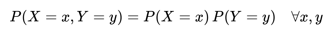
In other words, knowledge of X does not provide any information about Y, and vice versa. Independence implies no dependence of any kind, whether linear or non-linear, or even more complex relationships. It also implies zero correlation, but the reverse is not necessarily true.
Counter-Example Illustrating the Difference
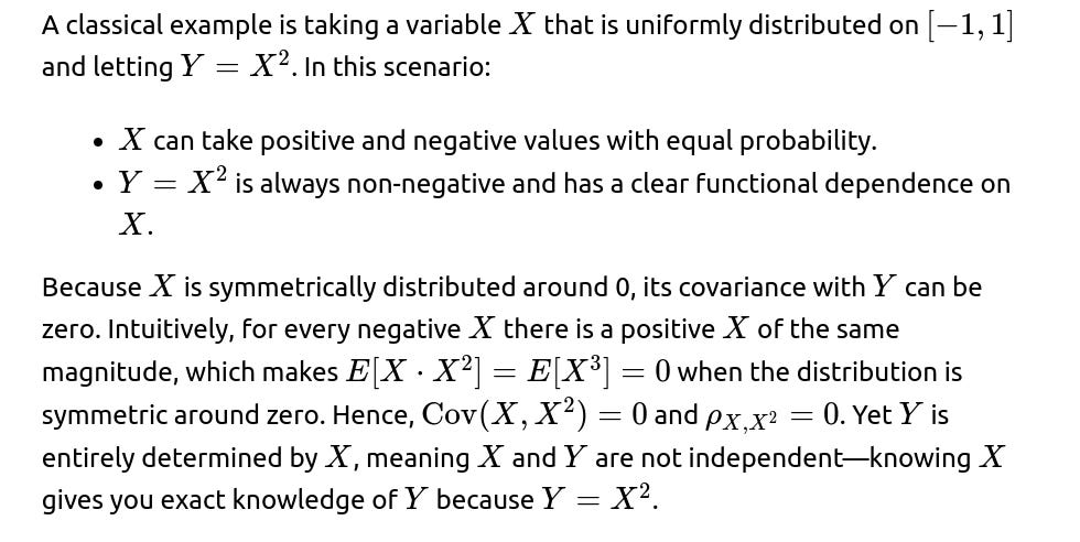
Therefore, zero correlation merely states there is no linear relationship, but there could still be a non-linear relationship that reflects genuine dependence.
Practical Relevance
In real-world data, you can easily have variables with complex dependencies. For instance, a variable might be related to the square, exponential, or logarithm of another variable. Standard correlation checks (like Pearson correlation) will not always detect such relationships.
To detect more general dependencies, you would look at higher-order statistics or use mutual information, kernel-based measures (like HSIC), or methods like distance correlation.
Follow-up Question 1
Why does independence always imply zero correlation, but zero correlation does not necessarily imply independence?
Because independence means that the joint distribution is completely factorizable into separate distributions of each variable. This complete factorization implies there is no way to predict one variable from the other, even via non-linear transformations. Consequently, all moments factorize, leading to a covariance of zero. However, having zero covariance only rules out linear relationships but does not exclude more general functional relationships or dependence. Hence, zero correlation is a much weaker condition than independence.
Follow-up Question 2
How does this phenomenon manifest in practice when analyzing real-world data?
In practical scenarios, you might compute correlation between two variables and find a near-zero value. If you prematurely conclude “these variables are unrelated,” you might miss strong non-linear effects. For instance, a stock market variable X and another market indicator Y might have zero correlation on paper, yet Y might respond to the absolute changes in X. If your analysis only looks at linear correlation, you could overlook a crucial risk factor. Therefore, advanced exploratory data analysis techniques—like plotting the variables, computing rank correlations (Spearman’s or Kendall’s), or using generalized correlation measures—are often used.
Follow-up Question 3
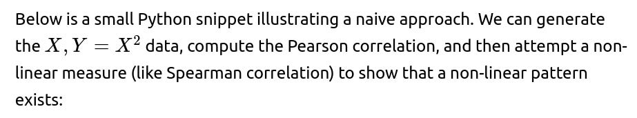
Could you give an example of how to code a quick check for non-linear dependence in Python?
import numpy as np
from scipy.stats import pearsonr, spearmanr

np.random.seed(42)

# Generate X uniformly in [-1,1]
X = np.random.uniform(-1, 1, 10000)
Y = X**2

# Pearson correlation (linear)
pearson_corr, _ = pearsonr(X, Y)

# Spearman correlation (rank-based, can detect some non-linear correlations)
spearman_corr, _ = spearmanr(X, Y)

print("Pearson correlation:", pearson_corr)
print("Spearman correlation:", spearman_corr)
Explanation of the code
We first create a large sample of size 10,000 from a uniform distribution in the interval [-1,1].
We define Y as the square of X.
We compute Pearson’s correlation with
pearsonr. Because of the symmetric nature of X, it should be near zero.We then compute Spearman’s rank correlation via
spearmanr. This measure can detect that Y grows with the magnitude of X, so you expect a non-trivial, positive Spearman correlation, indicating a dependence not captured by Pearson’s correlation.
Follow-up Question 4
Are there scenarios in which even advanced correlation measures might fail to capture certain dependences?
Yes. Some particularly pathological relationships or high-dimensional dependencies can be missed by standard correlation-based metrics (including rank-based measures). For instance, if the dependency is very subtle or only apparent in small pockets of the feature space, you might need specialized or domain-specific methods, or you could rely on generalized metrics like mutual information or other information-theoretic measures. In higher dimensions, the “curse of dimensionality” can also obscure dependence, requiring more sophisticated dimensionality reduction or specialized algorithms.
Follow-up Question 5
If we see zero correlation, what steps can we take in practice to confirm or refute independence?
Visual Inspection: Always plot your variables in scatter plots. Sometimes you will visually identify a pattern that the correlation measure fails to quantify (like a parabolic or circular pattern).
Compute Alternative Dependence Measures: Spearman’s correlation, Kendall’s tau, distance correlation, HSIC, or mutual information can give broader insight.
Hypothesis Testing: Use independence tests. There are many advanced statistical approaches (like kernel-based tests) that can directly test the hypothesis of independence.
Follow-up Question 6
What can happen if someone incorrectly assumes zero correlation implies independence in a machine learning pipeline?
If you incorrectly treat two variables as “safe to consider independent,” you might apply modeling or feature engineering decisions that ignore strong non-linear interactions. For example, you might throw away a feature because its correlation with the target is zero, yet in reality the feature has a significant non-linear effect that a complex model (like a neural network or random forest) could have exploited. This can lead to suboptimal model performance, overlooked predictive power, or incorrect inferences in statistical models.
Follow-up Question 7
How might this affect feature selection or dimensionality reduction steps in deep learning models?
In many deep learning pipelines, automatic feature extraction might circumvent some of the pitfalls of ignoring non-linear relationships. However, if a human is performing feature selection upfront based on correlation thresholds, potentially valuable non-linear features might be discarded.
Dimensionality reduction techniques such as PCA rely on maximizing variance along principal components, which is inherently a linear method. If important non-linear relationships exist, PCA might not capture them well, so methods like kernel PCA or other manifold learning approaches (t-SNE, UMAP) might be more appropriate.
Follow-up Question 8
Could independence be proven if we only tested a finite set of correlations and transformations?
No. True statistical independence requires that every possible relationship between the variables is absent. Testing only a finite set of transformations—be it polynomial relationships or just rank correlations—cannot conclusively prove independence for all functional forms. One often resorts to domain knowledge or advanced non-parametric tests, but in strict theory, it is impossible to fully prove independence using only finite observational data without strong assumptions.
Follow-up Question 9
Are there real-world distributions where zero correlation but dependence frequently occurs?
Yes. Financial time series often exhibit relationships that are more evident in volatility (squared returns) rather than the raw returns themselves. For instance, raw returns over short intervals can appear to have near-zero correlation, yet their magnitudes or squares can show volatility clustering. Many cyclical or periodic phenomena (e.g., certain seasonal patterns) can also exhibit zero mean correlation but exhibit dependence in other ways (like phases aligning).
Below are additional follow-up questions
How do partial correlations factor into the idea that zero correlation does not imply independence?
Detailed Explanation of the Question Partial correlation attempts to measure the linear dependence between two variables while controlling for other variables in the dataset. Even if two variables X and Y have zero correlation when considered in isolation, it is possible that once we hold a third variable Z constant, there emerges a non-zero partial correlation or vice versa. The key point is that direct correlation (Pearson correlation) is only one perspective; partial correlation can uncover hidden relationships that are masked when all variables vary freely.
Why This Matters In practice, especially in multivariate settings, we rarely analyze only two variables in isolation. Controlling for confounding variables can reveal or mask important non-linear or even linear relationships that are not evident otherwise. A zero correlation in raw data might lead to an incorrect conclusion of independence unless we check partial correlations and other measures that account for additional factors.
Example Scenario Imagine a situation with three variables: X, Y, and Z. Suppose that Y depends strongly on Z, and X also depends strongly on Z. If that dependence has a particular structure (e.g., X and Y each vary linearly with Z but in opposite directions), X and Y might appear to have near-zero correlation. However, if you control for Z (via partial correlation), you might see a significant relationship between the residuals of X and Y once Z is held constant.
Pitfalls or Edge Cases A common pitfall is to measure simple correlation between X and Y, find zero or close to zero, and conclude no relationship exists. Failing to measure partial correlations in complex datasets can lead to overlooking variables that become relevant only under certain conditions.
What role does canonical correlation analysis play in detecting more subtle relationships among sets of variables?
Detailed Explanation of the Question Canonical correlation analysis (CCA) extends the concept of correlation to pairs of sets of variables. Instead of measuring the correlation between two single variables, CCA finds linear combinations of one set of variables and linear combinations of another set of variables that maximize their mutual correlation.
Relevance to the Zero Correlation vs. Independence Discussion If each variable in set 1 is individually zero-correlated with each variable in set 2, one might hastily conclude there is no relationship. However, it is possible that a certain combination (a linear mixture) of the variables in set 1 is highly correlated with another combination of variables in set 2. Zero pairwise correlation does not guarantee that no such linear combinations exist.
Example In many neuroscience or genomics applications, each data point might consist of dozens or hundreds of measurements. Canonical correlation can show that a weighted sum of some neural signals is strongly associated with a weighted sum of gene expression signals, even though any individual neural measurement has a near-zero correlation with any individual gene measurement.
Pitfalls or Edge Cases Interpreting canonical correlations can be non-trivial. If the dataset is high-dimensional with relatively few samples, spurious canonical correlations might appear. Proper regularization or dimensionality reduction might be needed before trusting the results.
Can non-linear transformations mask or artificially create correlations, and how does that relate to the zero-correlation vs. independence distinction?
Detailed Explanation of the Question Transformations (such as logarithms, exponentials, squaring, or even standardizing) can drastically alter the correlation structure of data. A transformation might introduce curvature or distort scale in a way that either inflates or deflates correlation.
Why This Matters When we discuss the difference between zero correlation and independence, transformations can obscure or highlight relationships. A variable pair may exhibit zero correlation in their raw forms, but a log-transform could reveal a linear relationship (and thus a non-zero correlation). Conversely, a poor transformation can mask an otherwise visible correlation.
Subtle Real-World Example Financial returns are often log-transformed because price-level correlations may differ drastically from returns-level correlations. If someone incorrectly applies or omits the log transform, they might find spurious correlations or miss real ones.
Pitfalls or Edge Cases In some data preprocessing pipelines, multiple transformations are applied without carefully inspecting how they affect correlation structure. This can lead to contradictory or misleading findings about which features are “correlated.”
How do we differentiate between correlation and causation in scenarios where variables might be dependent but exhibit zero correlation?
Detailed Explanation of the Question Causation implies that changes in one variable bring about changes in another. Correlation, on the other hand, measures only a relationship—whether linear or non-linear—without specifying direction or mechanism. When variables have zero correlation but remain dependent, it demonstrates how tricky it can be to deduce causal relationships from purely observational data.
Real-World Pitfall In time-series analysis of economic indicators, one might see zero correlation in raw data, but more sophisticated methods (like Granger causality, structural equation models, or domain-based logic) reveal a causal mechanism. Relying solely on correlation-based arguments can lead to erroneous policy or business decisions.
In multivariate data, how can two variables each be correlated with a third variable but not correlate with each other?
Detailed Explanation of the Question This situation arises when X and Y each correlate with Z but not with each other. Specifically, X could increase with Z, and Y could also increase with Z, but the link between X and Y is negligible once Z is factored out. This ties back to the concept of partial correlation and confounding.
Relation to Zero Correlation vs. Independence X and Y might appear uncorrelated overall. However, they may still exhibit a conditional dependence given Z. Zero correlation does not necessarily mean independence, nor does correlation with a shared third variable ensure a direct relationship between X and Y.
Practical Pitfall In medical data, cholesterol level (X) and blood pressure (Y) might each correlate strongly with age (Z), but not necessarily with each other. If an analysis lumps everything together and checks only for correlation between cholesterol and blood pressure, it may overlook the underlying influence of age.
Could zero correlation arise purely from sampling issues, and how do we check for that?
Detailed Explanation of the Question Small sample sizes or biased sampling can yield misleading correlation measures. With a limited or non-representative sample, the empirical correlation might hover near zero even if there is a real underlying dependence.
How to Address This Researchers often perform statistical significance tests or confidence interval estimations for correlation coefficients. For small sample sizes, non-parametric methods or robust sampling techniques may be needed. In large sample sizes, correlation estimates become more stable, but one can still face issues if the data is systematically biased (e.g., missing not at random).
Potential Edge Cases A dataset with heavy outliers could bring the sample correlation closer to zero, even though most of the data exhibits a clear positive or negative trend. It’s essential to visualize data and possibly remove or mitigate outliers before concluding zero correlation.
How might zero correlation but dependence appear when dealing with periodic or cyclical data (e.g., signals with different phases)?
Detailed Explanation of the Question Cyclical or periodic variables might be completely out of phase with each other. If one signal peaks when the other is at a trough, and they do so consistently, the linear correlation could be near zero over a full cycle. However, if you align the signals or examine time-lagged correlations, a clear dependence might emerge.
Real-World Example Seasonal effects in climate data: daily temperature and daily humidity might have complicated time-lag relationships. Over certain months, these variables appear negatively correlated, while in other months they appear positively correlated. Over the entire year, the net correlation might be near zero, yet they exhibit strong seasonal dependence.
Pitfalls If one lumps an entire year’s data together, the correlation might vanish. If an analyst incorrectly concludes independence, important cyclical relationships can be missed. Breaking the data into appropriate segments or looking at cross-correlation with time lags can reveal the hidden dependence.
Is there a scenario where a non-monotonic relationship leads to zero correlation, and can we detect it with rank-based methods?
Detailed Explanation of the Question A non-monotonic relationship might increase in one region of X’s domain but decrease in another region. One classic example is a sinusoidal relationship: Y=sin(X). Over a full period, the ups and downs can cancel out in a Pearson correlation sense, yielding zero.
Rank-Based Detection Spearman’s rank correlation captures monotonic relationships but not all non-monotonic ones. So if the relationship is strictly monotonic, Spearman’s correlation will detect it. But if the relationship oscillates multiple times, you might still see near-zero rank correlation while a clear pattern remains. You might need more sophisticated measures (e.g., distance correlation or mutual information).
Real-World Subtlety In many engineering or physics contexts, signals can have harmonics or be wave-like. If an analyst tries only Pearson or Spearman correlation, they might see zero or near-zero correlation. A time-domain or frequency-domain analysis would be more appropriate.
How can spurious correlations complicate our understanding of zero correlation vs. independence?
Detailed Explanation of the Question A spurious correlation is a false or coincidental statistical relationship that arises from chance or from confounding variables. Even though we’re primarily concerned with the case of zero correlation, spurious correlations are important to consider because they remind us how easily random patterns can be interpreted incorrectly. Likewise, an apparent zero correlation might also be spurious if, in a larger dataset or under different conditions, a correlation emerges.
Edge Cases If we sample certain time frames or subsets of data, we might see ephemeral correlations or ephemeral zero correlations. The real distribution might yield a stable dependence if we had more comprehensive data.
Practical Advice Always scrutinize your data collection method. Look at broader time frames or different sub-populations to see if the zero correlation persists or changes drastically.
Can domain-specific knowledge override a zero correlation measure when suspecting an underlying relationship?
Detailed Explanation of the Question Zero correlation is a purely statistical measure of linear association. Domain knowledge might suggest that a causal or functional mechanism must exist (for example, physical laws or biological pathways). Even if you observe zero correlation in a given dataset, the prior knowledge might lead you to suspect that data sampling issues, transformations, or confounding variables are obscuring the relationship.
Why This is Important In fields like physics, chemistry, biology, or engineering, prior theoretical frameworks can be more reliable than raw statistical measures. If a well-established theory indicates Y depends on X, but your data yields zero correlation, you should be skeptical about concluding independence.
Pitfalls Overreliance on domain knowledge without checking the data properly can lead to ignoring real anomalies. Conversely, blindly trusting the correlation coefficient can make you miss a scientifically justified relationship that is masked in your observed sample.