
ML Interview Q Series: Zero Covariance: Proof from Constant Conditional Expectation E(X|Y=y).
Browse all the Probability Interview Questions here.
Prove that cov(X,Y) = 0 if E(X | Y=y) does not depend on y
Short Compact solution
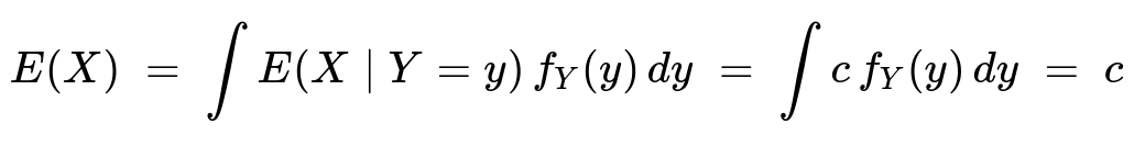
Let c be a constant such that E(X | Y=y) = c for every y. By the law of total expectation:
Next, by the law of total expectation applied to the product XY:
$$E(XY) ;=; \int E\bigl(XY ,\bigl|\bigr.,Y=y\bigr),f_{Y}(y),dy
;=; \int y,E\bigl(X ,\bigl|\bigr.,Y=y\bigr),f_{Y}(y),dy ;=; \int y,c,f_{Y}(y),dy ;=; c,E(Y)$$
Thus,
$$\mathrm{cov}(X,Y) ;=; E(XY);-;E(X),E(Y)
;=; c,E(Y);-;c,E(Y) ;=; 0$$
Comprehensive Explanation
When we say E(X | Y=y) does not depend on y, we are asserting that conditional on the event Y=y, the random variable X has the same expectation regardless of which particular value y takes. In other words, there is some constant c such that for every y, the average or expected value of X given that Y is y is always c.
From this, one can deduce two straightforward results:
E(X) = c. The law of total expectation states that E(X) = ∫ E(X | Y=y) f_Y(y) dy over all y in the support of Y. Because E(X | Y=y) = c, we can factor out c from the integral, and the remaining integral of the density f_Y(y) must be 1, so E(X) = c.
E(XY) = c E(Y). Again by the law of total expectation, we write E(XY) as ∫ E(XY | Y=y) f_Y(y) dy. Notice that E(XY | Y=y) = y E(X | Y=y), which is y c. Hence the integral becomes ∫ y c f_Y(y) dy = c E(Y).
Finally, to prove that the covariance is zero, recall that
cov(X, Y) = E(XY) - E(X) E(Y).
Since E(XY) = c E(Y) and E(X) = c, it follows that
cov(X, Y) = (c E(Y)) - (c E(Y)) = 0.
The intuition is that if, on average, X is unaffected by changes in Y (as indicated by E(X | Y=y) = constant), then X and Y have no linear dependence, resulting in zero covariance.
Potential Follow-up Questions
1) Could X and Y still be dependent even if cov(X, Y) = 0?
Yes, zero covariance only indicates that there is no linear relationship between X and Y. It does not necessarily imply independence. For example, X and Y can be non-linearly related and still have cov(X, Y) = 0. However, in this specific scenario where E(X | Y=y) is constant in y, it also implies a deeper kind of separation, often hinting that X might not be influenced by Y in a first-moment sense. But to claim full independence, we would need E(g(X) | Y=y) to be constant for all measurable functions g, which is a stronger condition than just E(X | Y=y) being constant.
2) Can E(X | Y=y) = c vary with a different function and still yield zero covariance?
If E(X | Y=y) were not a constant but some function of y, covariance need not be zero. Indeed, any correlation would emerge if E(X | Y=y) increases or decreases with y in a linear fashion, thereby changing E(XY). Having E(X | Y=y) = c (independent of y) is precisely the condition that forces the product E(XY) to factor into c times E(Y).
3) What if Y is a discrete random variable? Does the same proof apply?
Yes. The proof using sums instead of integrals is analogous. For a discrete Y taking values y_i with probabilities p_i, the law of total expectation says E(X) = ∑ E(X | Y=y_i) p_i. If E(X | Y=y_i) = c for all i, then clearly E(X) = c. Similarly, E(XY) = ∑ y_i E(X | Y=y_i) p_i = c ∑ y_i p_i = c E(Y), leading to zero covariance.
4) How might we verify this property numerically in a practical scenario?
In a computational setting, you could simulate many sample pairs (X, Y) from the joint distribution. Then:
Estimate E(X) by taking the average of all sample X values.
Estimate E(XY) as the average of the product X·Y over the sample.
Estimate E(Y) similarly.
Compute cov(X, Y) by cov(X, Y) = E(XY) - E(X) E(Y).
If in your simulations E(X | Y=y) is indeed constant, these estimates should converge to values that yield zero for the covariance. Of course, in finite samples one expects small numerical deviations, but with enough samples it should be very close to 0.
5) Are there any distributional assumptions necessary for this proof?
The primary assumption is that X and Y have well-defined expectations and that E(X | Y=y) is the same for all y. Beyond that, as long as we can apply the law of total expectation (and the integral or summation converges), there are no special distributional requirements. X and Y can be continuous, discrete, or mixed, as long as the integrals/sums for E(X) and E(XY) are properly defined.
6) Is it sufficient that E(X | Y=y) be almost surely a constant?
Yes. If E(X | Y=y) = c with probability 1, that is enough to carry over the entire argument. Covariance depends on expected values, so almost sure properties suffice. Even if there were a set of y values of measure zero where E(X | Y=y) might differ, it would not affect the integral or sum defining E(X) and E(XY).
7) Could the same argument be used to prove that E(Y | X=x) = constant implies cov(X,Y) = 0?
Absolutely. The roles of X and Y can be exchanged. If E(Y | X=x) is a constant for all x, a similar derivation shows that E(Y) is that constant, and E(XY) = E(X) E(Y), leading to zero covariance. The essence is that one variable’s conditional expectation does not vary with the other variable, removing any linear relationship.
8) If cov(X, Y) = 0, under what additional conditions can we say X and Y are independent?
A common additional condition is that (X, Y) is jointly Gaussian (i.e., normally distributed). In that special case, zero covariance implies independence. For general distributions that are not Gaussian, zero covariance alone does not guarantee independence. You would need stronger conditions, such as the entire conditional distribution of X given Y (and not just its mean) being independent of Y.
Below are additional follow-up questions
What if E(X | Y) = c but E(Y | X) is not constant? Does it still guarantee cov(X, Y) = 0?
If E(X | Y=y) = c for every y, we already know that cov(X, Y) = 0. However, this does not require that E(Y | X=x) also be a constant in x. The covariance depends on how X and Y co-vary overall, not on whether Y’s conditional expectation is or isn’t constant. For covariance purposes, the only necessary condition in this argument is that X’s conditional mean is invariant to Y. So even if E(Y | X=x) varies in some complicated way, that does not affect the conclusion that cov(X, Y) = 0, as long as E(X | Y=y) = c.
At an intuitive level, having E(X | Y=y) = c ensures that X has no systematic linear dependence on Y’s fluctuations. That is sufficient to drive covariance to zero, regardless of how Y might condition on X.
Can X still exhibit variability that depends on Y, even though E(X | Y=y) = c?
Yes. E(X | Y=y) = c only specifies that the mean of X does not change with y. It places no restrictions on higher-order moments such as var(X | Y=y). In other words, the conditional variance of X given Y=y could depend on y, making X distributionally different for different values of Y—even though its conditional mean remains the same constant c.
For instance, suppose X given Y=y follows a distribution with mean c but variance g(y), where g might be some function of y. In that scenario, the average value of X does not move with Y, but the spread (variance) might. Even so, the covariance is driven by how the linear component of X tracks Y in expectation, and that remains zero if the mean is constant.
How does having infinite or undefined variances or means affect this result?
The key requirement for the covariance formula to hold is that E(X), E(Y), and E(XY) all exist (i.e., they are finite). If either X or Y lacks a finite mean, then discussing E(X | Y=y) = c becomes delicate—because conditional expectation might not even be well-defined. Similarly, if E(XY) is not finite, the covariance is not well-defined.
Hence, the statement “if E(X | Y=y) = c, then cov(X, Y) = 0” presupposes that the necessary integrals converge so that the law of total expectation is valid and that the covariance is properly defined. If we encounter infinite or undefined expectations in a real-world problem, we cannot directly apply this result without additional conditions or transformations (e.g., truncation, transformations to ensure finite moments, etc.).
Is there a direct way to test if E(X | Y=y) = c in a practical data-driven scenario?
Testing E(X | Y=y) = c from data alone typically involves:
Partitioning the data based on different values (or bins) of Y.
Estimating the sample mean of X within each bin.
Checking whether those conditional sample means are statistically indistinguishable from a single constant.
For continuous Y, one might do a nonparametric regression of X on Y and see if the regression curve is essentially a flat line. Alternatively, one could set up a hypothesis test such as H0: “E(X | Y=y) = c for all y” versus HA: “E(X | Y=y) is not a constant.” In practice, measurement error, small sample sizes, or the presence of outliers can obscure whether E(X | Y=y) is truly constant or merely appears flat within sampling variability. So one must interpret the results carefully.
Can we extend this property to multiple variables, for instance if E(X | Y, Z) = constant?
If we have three variables X, Y, and Z, and we know that E(X | Y=y, Z=z) = c (independent of y and z), that directly tells us that in the presence of both Y and Z, X has a constant conditional mean. From that, one can similarly deduce that E(X) is c, and E(XYZ) factors in a certain way when conditioning on Y and Z. However, the question of cov(X, Y) = 0 or cov(X, Z) = 0 can be handled in a simpler way by marginalizing over the other variable. For instance, one could write:
E(XY) = E[ E(XY | Y, Z) ] = E[ Y E(X | Y, Z) ] = E[ Y c ] = c E(Y).
Hence cov(X, Y) = c E(Y) - c E(Y) = 0. A similar argument applies to Z. More generally, if E(X | Y1, Y2, ..., Yn) is constant, then X has zero covariance with any of those Y’s individually.
How does this relate to linear regression concepts?
In simple linear regression of X on Y, the slope coefficient is b = cov(X, Y) / var(Y). If E(X | Y=y) = c, then we already know cov(X, Y) = 0, which implies b = 0. Interpreting that in regression terms, it means the best linear predictor of X given Y is simply a constant (i.e., the intercept) and that variations in Y offer no explanatory power in predicting X.
This does not necessarily mean X and Y are independent. It only means that a linear model of X based on Y has no slope, so Y does not reduce the squared error of predicting X in a linear sense. There could still be a more complex nonlinear or “strange” dependence, but none that manifests in the first-moment (mean-based) relationship.
Could E(X | Y=y) be some “random constant” dependent on other variables not captured in Y?
Sometimes in more advanced setups, one might consider a hierarchical or multi-level model where there is another variable W. In that case, E(X | Y=y, W=w) could be c(w), a function of w, which might appear like a “random” constant once Y is considered in isolation. If we marginalize over W, that might or might not yield E(X | Y=y) = c.
Hence, it’s important to specify whether the statement “E(X | Y=y) = c” is unconditional with respect to every other variable. If so, it is truly a universal constant. If not, you may have something that looks like a constant in the Y dimension but is still varying across other dimensions, and that partial variation could lead to subtle dependencies.
What if Y’s domain is restricted or has boundary conditions?
If Y’s support is limited to a small interval or discrete set of values, E(X | Y=y) might trivially appear constant over that domain without necessarily implying independence. One subtlety arises when Y takes very few distinct values: you may not have enough information to confidently claim a functional relationship or lack thereof between X and Y. For instance, if Y can only be 0 or 1, and if E(X | Y=0) = E(X | Y=1), indeed you get zero covariance. But this is a special discrete scenario where you typically would confirm by direct calculation that the two conditional means coincide.
How does one handle cases where partial expectations exist but full expectations do not?
It is possible to have a situation where E(X | Y=y) is well-defined for each y (for example, it might be c), but integrating with respect to y to get E(X) might diverge if the support of Y extends to regions that give unbounded integrals. In that pathological case, statements about covariance become tricky because E(X) might not exist. You could have a scenario where each conditional expectation is finite, yet the marginal expectation diverges.
For standard probability distributions encountered in most statistical or machine-learning contexts, this situation is rare (and typically indicates a heavy-tailed distribution). But it is important to know that such theoretical pitfalls exist. In such unusual cases, we cannot properly speak of “cov(X, Y) = 0” because the covariance might not be well-defined.