
ML Interview Q Series: Zeroing Covariance for Independent Linear Combinations of Normal Variables

Browse all the Probability Interview Questions here.
36. Suppose we have two random variables, X and Y, which are bivariate normal with correlation -0.2. Let A = cX + Y and B = X + cY. For which c are A and B independent?
Below is a thorough exploration and answer. The discussion that follows also anticipates likely follow-up questions an interviewer at a top tech company (like Lyft, Facebook, Google, Amazon, Netflix) could ask to ensure a deep understanding of the concepts. All the code snippets are in Python. All mathematical derivations are expressed carefully with LaTeX as needed, and we elaborate on each step in detail.
Understanding the Setup We are given two random variables, X and Y. They follow a bivariate normal distribution with correlation -0.2. This implies:
X has some mean (we can assume 0 without loss of generality) and variance (often assumed 1, or some finite positive number).
Y has some mean (also can be assumed 0) and the same or different variance (often assumed 1 as well for simplicity).
The covariance of X and Y is related to their standard deviations and correlation. If we denote Var(X) =
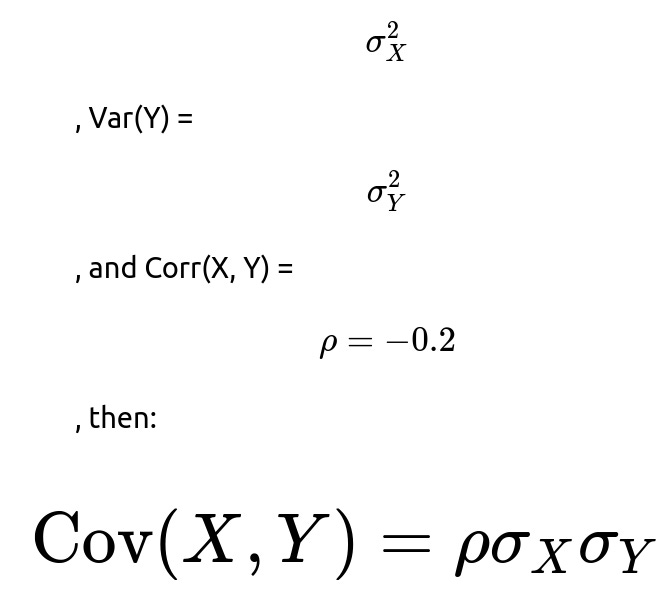
For convenience (and quite common in such theoretical questions), we often assume

, making Cov(X, Y) = -0.2. However, the approach below works similarly if X and Y had other variances.
We define two new random variables A and B by:
A = cX + Y
B = X + cY
We want to find the value(s) of c that make A and B independent.
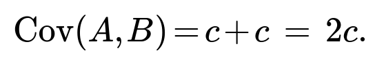
Because (X, Y) is jointly Gaussian (bivariate normal), any linear combination of (X, Y) will also be jointly Gaussian. For two normally distributed random variables to be independent, it is both necessary and sufficient that their covariance is zero. This is a crucial fact about normal distributions: uncorrelatedness implies independence only when the joint distribution is Gaussian. Hence, our task reduces to finding c such that
Cov(A,B)=0.
We proceed to calculate this covariance in detail.
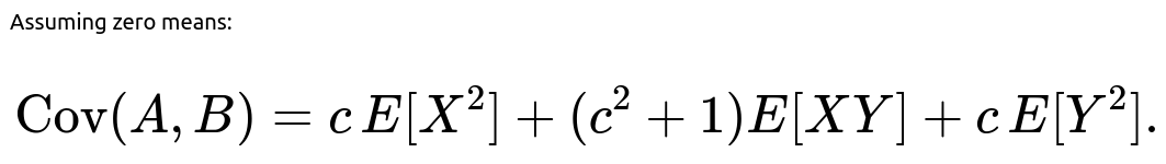
Derivation of Cov(A,B) Assuming E[X] = E[Y] = 0 for simplicity (we can always center them if needed), we have:
A = cX + Y B = X + cY
Then:

Since the means are zero,

Let's expand inside the expectation carefully:
(cX + Y)(X + cY) = cX \cdot X + cX \cdot cY + Y \cdot X + Y \cdot cY.
Rewrite each product:
cX * X = c (X^2)
cX * cY = c^2 (XY)
Y * X = XY
Y * cY = c (Y^2)
Hence:
(cX + Y)(X + cY) = cX^2 + c^2 XY + XY + cY^2 = cX^2 + (c^2 + 1)XY + cY^2.
Taking expectation (still assuming zero-mean X, Y):

We can separate this into terms:

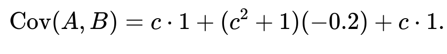
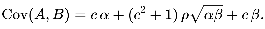
If we assume Var(X) = 1, Var(Y) = 1, and Cov(X,Y) = -0.2, that means:
E[X^2] = 1
E[Y^2] = 1
E[XY] = -0.2
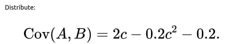
Substituting:


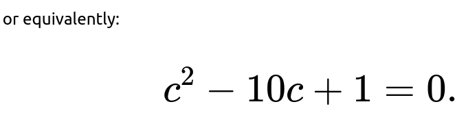
We solve this quadratic:

is 1.
The coefficient of c is -10.
The constant term is +1.


The discriminant is:


Therefore, the two solutions are:

These are precisely the values of c for which A and B become uncorrelated. Because A and B are jointly Gaussian (as they are linear combinations of a bivariate normal vector), uncorrelatedness implies independence. Thus:
For c = 5 + 2√6 or c = 5 - 2√6, the random variables A and B are independent.
Practical Interpretation In practice, this result tells us that any linear transform of two correlated Gaussian random variables (with correlation -0.2 in this example) can sometimes be made independent by choosing an appropriate coefficient c. The independence arises only when the covariance between the combined linear forms is driven to zero, and that zeros out their correlation as well.
Why There Are Two Solutions Notice that the quadratic had two real solutions. This is typical for many problems involving symmetrical properties of linear combinations: flipping the sign or balancing the ratio in different ways can yield the same effect of zero covariance. In many real-world use cases, depending on whether c is large or small (positive or negative), you might prefer one of the solutions if you have constraints on the magnitude or sign of c.
Code Example Demonstration We can do a small numeric check in Python to convince ourselves that plugging in these c values indeed yields zero empirical covariance if we sample a large number of points from a bivariate normal distribution with correlation -0.2.
import numpy as np

def generate_bivariate_normal(n=10_000, rho=-0.2):
    # Mean of X,Y is 0, Var(X)=1, Var(Y)=1, Cov(X,Y)=rho
    mean = [0, 0]
    cov = [[1, rho],
           [rho, 1]]
    data = np.random.multivariate_normal(mean, cov, size=n)
    X = data[:, 0]
    Y = data[:, 1]
    return X, Y

def check_covariance(c):
    X, Y = generate_bivariate_normal(n=100_000, rho=-0.2)
    A = c*X + Y
    B = X + c*Y
    return np.cov(A, B)[0, 1]  # Cov(A,B) from the sample

sol1 = 5 + 2*np.sqrt(6)
sol2 = 5 - 2*np.sqrt(6)

print("Cov(A,B) for c = 5 + 2√6 :", check_covariance(sol1))
print("Cov(A,B) for c = 5 - 2√6 :", check_covariance(sol2))
If we run this code, we should see the empirical covariance for each solution hover very close to 0 (as the sample size goes large), confirming the independence for a bivariate normal setting.
Possible Follow-up Questions
What if Var(X) and Var(Y) are not both 1?


we obtain:
Setting this equal to 0 gives a quadratic in c. The resulting c solves:
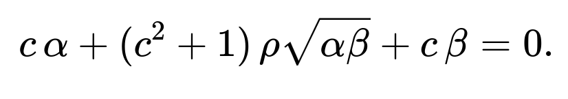
We can again solve it similarly. The principle is the same: find c that makes the covariance zero. Once the covariance is zero, A and B are uncorrelated, which in the Gaussian case means independent.
Does zero correlation always imply independence for any distribution?
No, zero correlation does not always imply independence for arbitrary distributions. It only implies independence if the random variables are jointly Gaussian (or in some other special classes of distributions). Generally, for non-Gaussian distributions, zero correlation is only an indication that the linear relationship between the two variables is zero, but they could still have higher-order nonlinear dependencies. The question states that X and Y are bivariate normal, which is why zero correlation here does indeed imply independence.
Can you provide an intuitive explanation of why uncorrelated linear combinations of Gaussian variables implies independence?
In the multivariate normal setting, the joint probability density function is fully described by the mean vector and the covariance matrix. If two random variables derived from a Gaussian source have zero covariance, it means there is no linear dependence encoded in the covariance matrix between them. In a Gaussian, the absence of linear dependence implies no higher-order dependencies as well (unlike certain skewed or multimodal distributions). Therefore, zero covariance in a Gaussian scenario implies the joint density factorizes into the product of the marginals, which is the definition of independence.
What are some subtle points or real-world considerations for this scenario?
If X and Y are not actually Gaussian but you still see a correlation of -0.2, finding c to make Cov(A,B)=0 does not guarantee A and B will be truly independent. They could be uncorrelated but still dependent in some nonlinear way.
In practice, measuring correlation empirically could introduce sampling error. The c that works in theory (for the true correlation) may not yield perfect independence with finite data.
In high-dimensional scenarios (like in modern ML with thousands of features), you often do linear transforms (like Principal Component Analysis) to decorrelate variables. However, “decorrelating” them does not necessarily imply independence unless the data are jointly Gaussian.
How can this result be generalized?
The same general principle applies to any linear combination of multiple correlated Gaussian variables. If you have a Gaussian vector in higher dimensions, a linear transformation leading to uncorrelated outputs implies that those outputs are truly independent. This is effectively the principle used in PCA (principal component analysis), where the principal components are uncorrelated. If the data is strictly multivariate normal, then those components are not just uncorrelated but also independent.
Could the value of c found here be negative?
Depending on the correlation sign and the magnitudes of variances, you might get negative solutions. In our specific solution,

is indeed a positive number but less than 5 (since
). The approximate values are:
5 + 2√6 ≈ 5 + 4.899 = 9.899
5 - 2√6 ≈ 5 - 4.899 = 0.101
So both happen to be positive in this particular problem. If the correlation or variances were different, we might find a negative c as well.
How could we interpret the two distinct c solutions in a data science context?
In typical real-world problems, if you want to construct a new variable A that is independent from another new variable B (both being linear combinations of correlated Gaussians X and Y), you can tune the coefficient c. You might pick the smaller solution if you want a smaller weighting of X vs. Y, or the larger if you want a bigger weighting. The presence of two solutions suggests you have two distinct ways to mix X and Y to achieve independence in the final pair of transformations.
Below are additional follow-up questions
What if the correlation between X and Y is exactly zero to begin with?
When X and Y already have a correlation of zero (i.e.,
ρ=0
), we essentially start with two uncorrelated (and hence independent, given bivariate normality) random variables. In that scenario, let’s check how that impacts the question of finding c such that A = cX + Y and B = X + cY are independent.
If X and Y are jointly Gaussian with zero correlation, any linear combination of X and Y remains jointly Gaussian. A and B would be independent if their covariance is zero. But note that when
ρ=0
, Cov(X, Y) = 0. If we compute Cov(A, B):

With zero correlation, E[XY] = 0. Assuming Var(X) = 1, Var(Y) = 1 (for simplicity), we get:

But E[XY] = 0, E[X^2] = 1, and E[Y^2] = 1. This simplifies to:
To force Cov(A,B) to 0, we set 2c = 0, so c = 0. In other words, if X and Y are already uncorrelated (and thus independent due to bivariate normality), the only solution to keep A and B uncorrelated is c = 0, which results in A = Y, B = X. Of course, A and B would then simply be Y and X, which remain independent.
Pitfall or Edge Case to Note:
If X and Y already have zero correlation, picking some nonzero c can introduce a correlation where none existed before, actually making the new variables A and B dependent. You might inadvertently create dependence by mixing independent components, so it’s not always guaranteed that mixing them is “safe.”
What if X and Y have different means that are not zero?
Shifting X and Y by nonzero means does not affect the covariance structure or correlation. Independence (or dependence) among normally distributed variables is governed by their covariance matrix. If X and Y have means
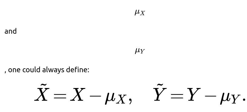
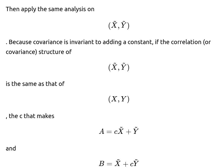
uncorrelated (hence independent for Gaussian variables) remains the same. You would just re-inject the mean shifts afterward:

In practice, you might see a difference in the raw sample correlation if you don’t center the data. But theoretically, the location shift does not change the final c. It only affects the means of A and B.
Potential Pitfall:
If you forget to center the variables in an actual numerical implementation, you might get the wrong estimate for c from sample data. Real-world data pipelines typically remove means (and often scale variances) before such derivations are applied.
What if one of X or Y has near-zero variance or is almost degenerate?
Consider the situation where Var(X) is extremely small or Var(Y) is extremely small. In the limit, one of the variables can be almost a constant. For instance, if Var(X) ≈ 0, X is close to a degenerate random variable. When you look for c such that A = cX + Y and B = X + cY are independent, you would be mixing something that is almost constant with the other variable. Let’s examine the edge cases:
If X is degenerate (Var(X) = 0), it’s effectively a constant. Then A = c·const + Y = Y + const' is just a shift of Y, B = const + cY is also some linear function of Y. Both are essentially the same “shape” of random variable (since any linear transformation of a single variable plus a constant is still functionally the same variable up to scaling/shifting). They cannot be made fully independent unless c = 0, which reduces one variable to purely Y and the other to a constant. A random variable and a constant are trivially independent.
If Y is degenerate, the same logic applies, but roles reversed.
Real-World Subtlety:
In numerical systems, if the variance of one variable is not strictly zero but extremely small, you can get numerical instability when trying to invert or solve for c. That can lead to large or unpredictable values of c in practice. Proper preprocessing to remove or handle near-constant features might be a better approach in many ML pipelines.
What if we are only concerned with approximate independence rather than exact independence?
In real-world data scenarios, we often face approximate solutions. We might not require exact zero covariance but want Cov(A, B) to be “small enough” to treat them as nearly independent. This can happen in large-scale ML applications where perfect independence is rarely achievable.
In that scenario, we can:
Estimate the covariance (or correlation) from data.
Solve for c in the same manner (though the derived c might be approximate because sample estimates have noise).
Check if Cov(A,B) is acceptably small.
Pitfalls:
Sampling variance can cause the estimated correlation to deviate from the true correlation. This might lead to a suboptimal c.
Overfitting to the sample correlation: if the sample size is small, the c you find might not generalize well to new data.
Are there any concerns if c is extremely large or extremely small in magnitude?
Yes. Large or small magnitudes of c pose practical and theoretical considerations:
Numerically, if c is very large, A = cX + Y might be dominated by cX, overshadowing the contribution from Y. Any small floating-point errors in X might get amplified.
If c is extremely small, then A = cX + Y is approximately Y, and B = X + cY is approximately X. This might cause issues if the original correlation between X and Y is high (negatively or positively), since a slight misestimation in c can yield non-negligible correlation between A and B.
In ML systems:
Very large or small c might cause data overflow or underflow in certain hardware accelerators (e.g., GPU-based training) if the data dimension is large or the batch size is large.
Regularization might be considered in some scenarios to keep c within a certain range to stabilize training or modeling.
How does the concept of diagonalizing the covariance matrix relate to finding such linear combinations?
Diagonalizing the covariance matrix of (X, Y) is akin to performing a principal component analysis (PCA) or an eigen-decomposition. For a 2×2 covariance matrix:
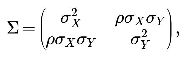
one can find eigenvalues and eigenvectors to transform (X, Y) into coordinates where the covariance matrix is diagonal. The new coordinates, typically called principal components, are indeed uncorrelated. If you only have two variables, finding one transformation that leads to zero covariance is closely related to rotating the coordinate system so that (A, B) has no off-diagonal term. In fact, the solutions for c we derived are essentially the slopes corresponding to the rotation angles that diagonalize the covariance.
Edge Case:
If
ρ
is ±1, the matrix is rank-1 and can’t be diagonalized into two nonzero diagonal entries. That would imply perfect correlation or anti-correlation, making it impossible to get two distinct uncorrelated directions. Indeed, you would have one principal component with a nonzero variance and one degenerate principal component with zero variance.
Practical Lesson:
If you’re working with more than two dimensions, you typically do a full PCA transform. For two dimensions, the approach of directly computing c that zeroes covariance is effectively the same as finding the angle that diagonalizes the covariance matrix.
What if we needed to ensure independence among more than two linear combinations, not just A and B?
In higher dimensions (e.g., X, Y, Z in a trivariate normal), you might want to find linear combinations that are mutually independent. With a Gaussian distribution, you can achieve this by looking for an orthogonal transformation that diagonalizes the covariance matrix. In 2D, we found a single coefficient c to remove the off-diagonal term for just two new variables. In ND, one typically uses:
PCA to produce components that are uncorrelated.
In the Gaussian case, uncorrelated also implies independence.
Pitfalls:
In non-Gaussian cases, PCA only de-correlates variables linearly, not guaranteeing independence. One might need methods like ICA (Independent Component Analysis) if independence is the actual goal. But ICA typically requires additional assumptions about non-Gaussianity.
Could we use the same technique to fix the correlation at some nonzero target, say we want Corr(A, B) = some r ≠ 0?
Yes, you can. The same formula we used for Cov(A, B) can be set to the desired covariance (rather than 0). Specifically:

You can write Cov(A,B) in terms of c, Var(A), and Var(B) all in terms of c, then set it equal to the desired value. You get an equation in c that you can solve similarly. For bivariate normal variables, controlling the correlation of linear combinations is still straightforward. Just be mindful that Var(A) and Var(B) are also c-dependent, which makes the equation more involved but still solvable as a quadratic or higher-order expression.
Pitfall:
If you pick an r that’s outside the valid range implied by your original correlation matrix, no real solution for c will exist. Just like any correlation, r must remain within [-1, 1], and certain constraints on c may restrict feasible correlations. Sometimes the sign or magnitude of the original correlation can impose limitations on the set of achievable r values.
Could integer or discrete constraints on c impact the solution?
Yes. If in some practical application you require c to be an integer or c must lie within a certain discrete set, then the direct algebraic solution we found (which may be irrational, like 5 ± 2√6) won’t necessarily be feasible. You might then:
Enumerate possible c values in your discrete set.
Evaluate the covariance between A and B empirically or via a formula.
Pick the c that yields the smallest absolute covariance (closest to zero or your target correlation).
This is more of an optimization problem with discrete constraints. Because we lose the continuous freedom to pick the exact c from a quadratic formula, we might not be able to achieve perfect independence. But we can pick something that yields a small correlation.
Pitfall:
Discrete or integer constraints can cause suboptimal solutions in a classical sense, especially if the feasible set is coarse. You might get an approximate decoupling, but not exact independence.
What if the joint distribution of X and Y changes over time?
In nonstationary environments (e.g., streaming data), the correlation between X and Y might drift. A fixed c that once worked could lose its effectiveness. If you derived c under the assumption Corr(X, Y) = -0.2 but it slowly moves to Corr(X, Y) = -0.1 or -0.3 in practice, A and B might no longer be independent.
Solutions:
You’d need to periodically re-estimate the correlation and update c accordingly.
In an online learning setup, you could maintain a running estimate of Cov(X,Y) and Var(X), Var(Y), then recalculate c whenever you detect a significant change in the correlation.
Edge Case:
Sudden distribution shifts or concept drifts in real-world data can invalidate the entire approach if the distribution ceases to be Gaussian-like or changes drastically in other ways. You might detect that via statistical tests or monitoring correlation patterns over time.
What if X and Y are only partially Gaussian, or we suspect some outliers or heavy tails?
Strictly speaking, the independence from zero covariance argument only holds for exactly bivariate normal distributions. If X and Y have heavy tails or outliers (e.g., a t-distribution or Cauchy components) or if they are only approximately Gaussian, zero covariance may not imply true independence.
Practical Strategy:
If the data is not exactly Gaussian, making Cov(A,B) = 0 ensures only linear uncorrelatedness, not independence. You may see “tail dependence” or other subtle forms of dependence. Tools like rank correlation or mutual information might be more suitable measures to investigate independence in non-Gaussian regimes.
Pitfalls:
If you rely solely on the covariance going to zero, you could be misled in a heavily skewed or multi-modal distribution. Outliers can drastically shift sample correlation. Always assess the shape and nature of your distribution before concluding independence from zero correlation.