ML Interview Q Series:Can you explain how you might modify a regression loss function to explicitly penalize large negative predictions more than large positive ones in a revenue forecasting scenario?

📚 Browse the full ML Interview series here.

Hint: Asymmetric cost functions, such as a tilted loss, can weigh errors differently.

Comprehensive Explanation

In many revenue forecasting situations, underestimating revenue can have more severe consequences than overestimating it. This leads to the desire for a loss function that penalizes negative errors (i.e., actual value minus predicted value, if the prediction is smaller than actual) more than positive errors. A classical approach is to use an asymmetric cost function that assigns different weights depending on whether the model overpredicts or underpredicts.

One prominent example is the tilted loss, sometimes called the “quantile loss” or “pinball loss.” The essence is to introduce a parameter (often denoted by alpha in text form) that adjusts how heavily we penalize positive versus negative errors. This alpha in text form can range from 0 to 1, determining whether we care more about underestimates or overestimates.

Below is the core mathematical expression in big font, showing an example of an asymmetric (tilted) loss function for a single observation:

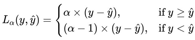
This expression can be read in text form as follows: If the actual y is greater than or equal to the prediction y_hat, the loss is alpha * (y - y_hat). Otherwise, the loss is (alpha - 1)*(y - y_hat). Notice that if alpha is greater than 0.5, the cost of underestimating is more severe than overestimating.

The parameters of the above formula are:

• y is the actual target value (revenue in this scenario).

• y_hat is the predicted value from the model.

• alpha (in text form) is a scalar in the interval (0, 1) that governs how much to weigh positive versus negative deviations. For instance, if alpha=0.8, the cost of underestimating by a certain margin is 0.8 times that margin, whereas the cost of overestimating by the same margin is only 0.2 times that margin (because alpha-1=-0.2).

This asymmetric property allows you to penalize large negative predictions more heavily, thereby aligning more closely with use cases where underestimates are riskier. You can adjust alpha to reflect how much you want to penalize negative errors relative to positive ones.

Practical Implementation

To use this asymmetric loss in a deep learning framework like PyTorch, you can write a custom loss function. For instance:

import torch
import torch.nn as nn

class AsymmetricTiltedLoss(nn.Module):
    def __init__(self, alpha=0.8):
        super(AsymmetricTiltedLoss, self).__init__()
        self.alpha = alpha

    def forward(self, y_pred, y_true):
        # y_pred and y_true should be tensors of the same shape
        diff = y_true - y_pred
        mask = (diff >= 0).float()  # 1 if y_true >= y_pred, 0 otherwise
        loss = self.alpha * diff * mask + (self.alpha - 1) * diff * (1 - mask)
        return torch.mean(loss)

In this code:

• We compute diff = y_true - y_pred in text form.

• If the difference is non-negative, we multiply by alpha in text form.

• If the difference is negative, we multiply by alpha - 1 in text form, making the sign negative and thus less penalizing if the prediction overshoots.

By setting alpha to a value larger than 0.5, you explicitly penalize underestimates more strongly.

Another Potential Follow-up Question

How do you choose the value of alpha in a tilted loss for your revenue forecasting model?

It is typically determined by the business context. If underestimates are severely detrimental, pick alpha closer to 1. If overestimates are more costly, pick alpha closer to 0.5 or even below 0.5. You can also use cross-validation or a validation set to empirically select the alpha that yields the best performance according to your chosen metric. In practice, one might iterate through different alpha values, compute the overall cost or performance metric, and select the best alpha.

Another Potential Follow-up Question

Can you explain the difference between a tilted loss and the standard Mean Squared Error (MSE)?

Mean Squared Error (MSE) treats positive and negative residuals (y - y_hat in text form) the same way. Squaring the error penalizes large deviations severely but does not allow you to differentiate how an overestimate or an underestimate affects your outcome. Tilted loss, on the other hand, is designed to be asymmetric, enabling you to weigh negative and positive deviations differently. This is crucial when the business scenario has different costs associated with overpredicting and underpredicting.

Another Potential Follow-up Question

What if we have outliers in our revenue data? How does the tilted loss compare to other robust losses like Huber?

Tilted loss focuses on asymmetry rather than outlier robustness. Huber loss is a compromise between L1 (absolute) and L2 (squared) norms to be more robust to outliers. Tilted loss, by contrast, is not explicitly robust against outliers; it is still linear in the error (except for the change in slope at zero). If outliers are a concern, one might combine approaches, like using a hybrid that incorporates asymmetry for negative/positive errors but also caps extreme values with a robust formulation. In practice, data preprocessing or outlier handling can be performed before applying the tilted loss function.

Another Potential Follow-up Question

Are there any optimization challenges with an asymmetric loss?

Yes, especially in gradient-based methods. The tilted loss is not differentiable at the point where y = y_hat in text form (the absolute “kink” in the piecewise function). However, in practice, frameworks like PyTorch can handle this with subgradient methods, and optimization typically remains stable. If you see convergence issues, you might try smoothing the absolute value (for example, using a small band around zero to approximate the kink smoothly).

Another Potential Follow-up Question

How can we combine this asymmetric loss with regularization?

Regularization is generally orthogonal to the choice of loss function in the sense that you can apply L2 or L1 penalties on the model parameters in parallel with the tilted loss. In frameworks like PyTorch, you can add weight decay to the optimizer, or you can manually add regularization terms (like the L2 norm of the weights) to the overall loss, summing them up with the asymmetric term. The choice of regularization coefficients depends on model complexity, data size, and the risk of overfitting.

Such a combination might look like:

loss = tilted_loss(output, target) + lambda_reg * torch.sum(model_params**2)

where lambda_reg in text form is a hyperparameter controlling the regularization strength.

All these considerations help ensure that your final model not only penalizes large negative predictions more than large positive ones but is also well-tuned and robust under various real-world conditions.

Below are additional follow-up questions

How can scaling or normalization affect the tilted loss, and what should be considered before applying it?

Scaling can significantly influence how a tilted loss function operates because any distortion in magnitude may skew the penalty differently for overestimates versus underestimates. If the data is very large (e.g., revenue in the billions) or very small (e.g., fractional revenues in specialized contexts), the tilt in the loss may become exaggerated or negligible, respectively.

One potential pitfall is when you apply a standard scaler or min-max normalization to the target variable y, but forget to reinterpret alpha in that normalized space. If underestimates in the original scale are much more severe, but you have normalized the data to [0,1], you could unintentionally dilute the penalty for underestimates. Alternatively, if you keep data unscaled, large absolute values might explode the gradient for negative or positive errors, potentially making training unstable.

To address these issues:

• Consistently apply scaling to both the target y and the predictions y_hat.

• Calibrate alpha carefully after scaling. The cost ratio implied by alpha might shift if the scale changes.

• Monitor gradients during training to detect if large magnitudes lead to exploding or vanishing gradients.

• Consider domain-specific post-processing: you might prefer training with normalized data for stability but convert predictions back to the original scale before final evaluation or decision-making.

What if we want to penalize sustained underestimation or overestimation across multiple predictions, rather than at a single point?

Tilted loss is typically applied on a per-sample basis, summing (or averaging) over all points in a dataset. However, if you want to penalize consistent underestimation over time (e.g., a time series of revenue forecasts), you might incorporate additional terms or constraints that look at aggregated errors across multiple time steps.

A potential approach is:

• Compute the tilted loss per time step and then sum or average.

• Add an additional penalty term on cumulative under-forecasts (like a separate measure of how often or how severely the model underestimates consecutively).

A pitfall is that introducing a temporal or cumulative penalty can make the optimization more complicated, potentially leading to instability in gradient-based methods. You need to balance the per-sample penalty (local perspective) with the multi-step penalty (global perspective). Also, if your data has seasonality or trend, a naive cumulative penalty may over-penalize normal cyclical dips, so you might want to incorporate domain knowledge or decomposition techniques to handle these seasonality factors.

How do we handle highly imbalanced datasets where some segments of the data require stronger penalties for negative errors than others?

Even within a single revenue dataset, certain segments (e.g., high-value customers or critical business units) might require a higher penalty for underestimation than others. You can extend the idea of a tilted loss by introducing weights that depend on data segments or business contexts.

For example:

• You could multiply the tilted loss by a weight w_i that depends on the importance of sample i.

• You could define alpha_i for different segments to reflect varying asymmetric sensitivities.

However, this can introduce complexity and may require more hyperparameters (separate alpha or weighting factors per segment). It’s critical to ensure that you have enough data in each segment to reliably learn an appropriate tilt. Otherwise, you risk overfitting to segments with fewer samples. An additional pitfall is interpretability: different alpha_i for different segments can make it hard to explain the overall behavior of the model to stakeholders unless you carefully communicate the rationale for segment-based weighting.

How do you address situations where the model might produce negative forecasts for inherently positive quantities like revenue?

Revenue is typically non-negative. When training a model with a standard regression approach (e.g., linear regression, neural networks with no output activation), it’s possible to predict negative values. This can cause confusion when the target is always positive. In the context of a tilted loss, a negative prediction leading to a large difference y - y_hat might be severely penalized if alpha is close to 1, which could push the model away from negative outputs over time.

Nevertheless, a few pitfalls might arise:

• A single large negative prediction might dramatically shift model parameters if the learning rate is high, causing instability.

• If the model architecture has no explicit constraint on positivity, certain optimization paths might meander around negative values.

Potential solutions include:

• Constraining the output to be positive, for example using a log transform of the revenue or applying a positivity-enforcing activation (e.g., ReLU or softplus).

• Applying careful preprocessing: modeling log(revenue) typically ensures the model output is unconstrained, but exponentiating the final predictions ensures positivity.

Could an excessively large alpha cause the model to always overshoot and remain biased upward?

Yes. If alpha is set extremely high, the penalty for underestimation dwarfs the penalty for overestimation. The model may learn a strategy that persistently overshoots the actual values, preferring the less severe penalty for positive errors. This can lead to consistent bias above the true values.

Why is that a pitfall? In some businesses, overestimating revenue might yield resource misallocation (e.g., overspending on operations). Thus, picking alpha too large can create new problems even though underestimates were initially the bigger concern. The solution is typically a more moderate alpha that balances the cost of underestimation with realistic tolerance for overestimation, possibly found via data-driven experimentation or explicit cost considerations. Careful monitoring of over-forecast bias through validation sets or domain-specific metrics is essential.

What if the revenue forecasting problem is multi-output (e.g., forecasting multiple types of revenue streams simultaneously)?

In multi-output scenarios, you might have multiple revenue streams (say from different product lines) predicted jointly. You can extend the tilted loss to handle vectors of predictions. Typically, you sum or average the tilted losses across each dimension, applying the same alpha for each. However, if different revenue streams have different cost asymmetries, you could assign distinct alpha_j for each revenue stream j.

Pitfalls include:

• Ensuring the scale and importance of each revenue stream is appropriately reflected. One high-volume revenue stream might dominate the overall gradient if it is far larger in magnitude than the others.

• Deciding whether each output dimension has its own alpha_j or whether you use a single alpha across all outputs, which might not capture domain-specific asymmetries.

When should we consider more advanced or custom asymmetric losses over the standard tilted (quantile) loss approach?

While the tilted loss is the most common asymmetric loss, advanced scenarios might require custom modifications:

• Situations where you care about percentage errors more than absolute errors. In that case, you might adapt the tilted loss to relative errors: alpha * (relative error) if y >= y_hat, etc.

• Risk management contexts where extremely large underestimates are exponentially more damaging. A custom exponential penalty might be considered.

• Complex business rules specifying threshold-based penalties: e.g., no penalty if you are within ±x% but penalize heavily beyond that.

The pitfall is that designing a more specialized loss can drastically complicate optimization. Such functions might be non-smooth or non-convex in ways that degrade gradient-based training. Also, custom-coded losses must be thoroughly tested to ensure correctness and stability in practice.

Are there any stability concerns if we combine the tilted loss with advanced optimization techniques like adaptive learning rates (e.g., Adam, RMSProp)?

Yes. Adaptive optimizers dynamically adjust the learning rate based on gradient history. When combined with the piecewise nature of tilted loss, if alpha is large, the gradient might spike whenever the prediction crosses from overestimating to underestimating. Adam might handle this effectively by adjusting step sizes, but sudden shifts can still lead to oscillations or slow convergence if the hyperparameters (beta1, beta2, learning rate) are not tuned carefully.

Potential strategies include:

• Conducting a hyperparameter search for the optimizer specifically around alpha ranges to ensure stable convergence.

• Employing gradient clipping to limit very large updates when alpha is close to 1.

• Monitoring training loss curves to identify instability (e.g., the loss bouncing or failing to steadily decrease).

Ultimately, stable convergence is achievable but demands some additional vigilance when using a loss function that has discontinuous derivatives or strong asymmetries.

How do we evaluate model performance when using an asymmetric loss?

Standard metrics like MSE or MAE (mean absolute error) might not accurately reflect your cost preferences if your training loss is strongly asymmetric. Evaluating only with MSE or MAE could obscure the real impact of large negative errors.

You may:

• Use the same tilted loss on a held-out validation set to see how the model performs in terms of your cost function of interest.

• Complement it with standard metrics to maintain comparability with other models or baselines.

• Incorporate domain-specific KPIs, for instance how many times you underforecast by more than a certain threshold, or the percentage of time you severely under-forecast.

A pitfall here is that if you rely solely on standard symmetric metrics while training an asymmetric model, you might not see the true cost improvements. Conversely, if you only use the tilted loss metric, you could lose broader perspective. A balanced approach is essential to see both the business-driven benefit and the usual metrics used in model benchmarking.