
Python Most Common Challenges

Interview Common Problems

Link to Kaggle Notebook for all these exercises together
Q: convert-decimal-to-binary
Performing Short Division by Two with Remainder (For integer part)
This is a straightforward method which involve dividing the number to be converted. Let decimal number is N then divide this number from 2 because base of binary number system is 2. Note down the value of remainder, which will be either 0 or 1. Again divide remaining decimal number till it became 0 and note every remainder of every step. Then write remainders from bottom to up (or in reverse order), which will be equivalent binary number of given decimal number. This is procedure for converting an integer decimal number, algorithm is given below.
Take decimal number as dividend.
Divide this number by 2 (2 is base of binary so divisor here).
Store the remainder in an array (it will be either 0 or 1 because of divisor 2).
Repeat the above two steps until the number is greater than zero.
Print the array in reverse order (which will be equivalent binary number of given decimal number).
Note that dividend (here given decimal number) is the number being divided, the divisor (here base of binary, i.e., 2) in the number by which the dividend is divided, and quotient (remaining divided decimal number) is the result of the division.
Example for number = 112
Divisision Remainder (R)
112 / 2 = 56 Remainder-0
56 / 2 = Remainder-28 0
28 / 2 = Remainder-14 0
14 / 2 = Remainder-7 0
7 / 2 = 3 Remainder-1
3 / 2 = 1 Remainder-1
1 / 2 = 0 Remainder-1
Now, write remainder from bottom to up (in reverse order), this will be 1110000 which is equivalent binary number of decimal integer 112.
def decimal_to_binary(_number_):
   if number == 0:
     return ""
   else:
    print(number)
    return decimal_to_binary(number // 2) + _str_(number % 2)

print(decimal_to_binary(112))

### In Python, you can simply use the bin() function to convert from a decimal value to its corresponding binary value._

### And similarly, the int() function to convert a binary to its decimal value. The int() function takes as second argument the base of the number to be converted, which is 2 in case of binary numbers._

### print(bin(112))  # 0b1110000_

# print(int('0b1110000', 2))_
Q: Product of two matrices
Given two matrices print the product of those two matrices
Solution with Explanations and Theory
Basics of Matrix Multiplication
Multiplication rule to remember — Here also the flow is Row and then Column
Sum-Product of First Row * 1st Column => Becomes the 1-st_Row-1-st_Column of the resultant Matrix
Sum-Product of 1st Row * 2-nd Column => Becomes the 1-st_Row-2-nd_Column of the resultant Matrix
There are four simple rules that will help us in multiplying matrices, listed here:
1. Firstly, we can only multiply two matrices when the number of columns in matrix A is equal to the number of rows in matrix B.
2. Secondly, the first row of matrix A multiplied by the first column of matrix B gives us the first element in the matrix AB, and so on.
3. Thirdly, when multiplying, order matters — specifically, AB ≠ BA.
4. Lastly, the element at row i, column j is the product of the ith row of matrix A and the jth column of matrix B.
Further read through this for a very nice visual flow of Matrix Multiplication.
# This works in O(n^3)_
def multiply_matrix(matrix1,matrix2):
    results = []
    try:
        for i **in** range(len(matrix1)):
            rows = []
            for j **in** range(len(matrix2[0])):
                item = 0
                for k **in** range(len(matrix1[0])):
                    item += matrix1[i][k] * matrix2[k][j]
                rows.append(item)
            results.append(rows)
        return results
    except:
        return "These matrices aren't compatible."
A1 = [[1, 2],
      [3, 4]]

B1 = [[1, 2, 3, 4, 5],
      [5, 6, 7, 8, 9]]


print(multiply_matrix(A1, B1))

# [[11, 14, 17, 20, 23], [23, 30, 37, 44, 51]]_
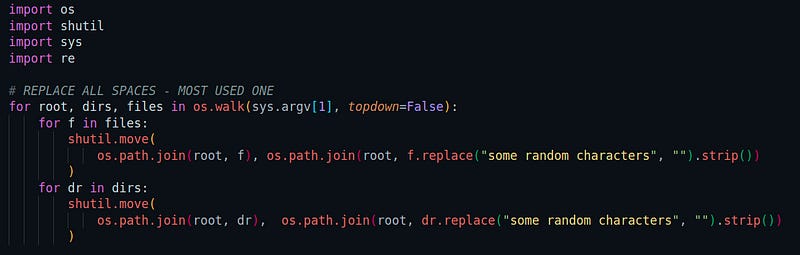
Replace characters from file-name
Q: Proportional Probability Sampling
Select a number randomly with probability proportional to its magnitude from the given array of n elements
consider an experiment, selecting an element from the list A randomly with probability proportional to its magnitude. assume we are doing the same experiment for 100 times with replacement, in each experiment you will print a number that is selected randomly from A.
Ex 1: A = [1, 5, 27, 6, 13, 28, 100, 45, 10, 79] let f(x) denote the number of times x getting selected in 100 experiments. f(100) > f(79) > f(45) > f(28) > f(27) > f(13) > f(10) > f(6) > f(5) > f(0)
Solution and Explanations and Notes on methods, steps, algorithms
The below solution is inspired by the explanations given in this Stackoverflow question.com
To explain further on the question -
I have an array of doubles and I want to select a value from it with the probability of each value being selected being proportional to its value. For example:
arr[0] = 100arr[1] = 200
In this example, element 0 would have a 66% of being selected and element 1 a 33% chance.
The general algorithm is
sum the array
Pick a random number between 0 and the sum
Accumulate the values starting from the beginning of the array until you are >= to the random value.
Note: All values must be positive for this to work.
The usual technique is to transform the array into an array of cumulative sums:
[10 60 5 25] --> [10 70 75 100]
Pick a random number in the range from zero up to the cumulative total (in the example: 0 <= x < 100). Then, use bisection on the cumulative array to locate the index into the original array:
Random variable x Index in the Cumulative Array Value in Original Array----------------- ----------------------------- ---------------------- 0 <= x < 10 0 1010 <= x < 70 1 6070 <= x < 75 2 575 <= x < 100 3 25
For example, if the random variable x is 4, bisecting the cumulative array gives a position index of 0 which corresponds to 10 in the original array.
And, if the random variable x is 72, bisecting the cumulative array gives a position index of 2 which corresponds to 5 in the original array.
For an inverse proportion, the technique is exactly the same except you perform an initial transformation of the array into its reciprocals and then build the cumulative sum array:
[10 60 5 25] --> [1/10 1/60 1/5 1/25] --> [1/10 7/60 19/60 107/300]
The actual function
import random

def pick_num_from_list(A):
    sum=0
    cum_sum=[]
    for i **in** range(len(A)):
        sum = sum + A[i]
        cum_sum.append(sum)
    #print(cum_sum)_
    r = int(random.uniform(0,sum))
    print(r)
    number=0
    for index **in** range(len(cum_sum)):
        if(r>=cum_sum[index] **and** r<cum_sum[index+1]):
            return A[index+1]
    return number

def sampling_connected_to_magnitued():
    # A = [0,5,27,6,13,28,100,45,10,79]_
    A = [1, 5, 27, 6, 13, 28, 100, 45, 10, 79]
    a = dict()
    #A.sort()_
    print(A,sum(A))
    for i **in** range(1,100):
        number = pick_num_from_list(A)
        #print(number)_
        if number **not** **in** a:
            a[number] = 1
        else:
            a[number]+=1
    print(a)


sampling_connected_to_magnitued()
Q: Closest points (based on Cosine Distance)
Find the closest points (based on cosine distance) in S (which is n data points in the form of list of tuples) from P (which is a point P=(p,q) )
Consider you have given n data points in the form of list of tuples like
S=[(x1,y1),(x2,y2),(x3,y3),(x4,y4),(x5,y5),..,(xn,yn)] and a point P=(p,q)
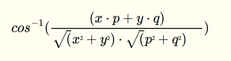
Your task is to find 5 closest points(based on cosine distance) in S from P
cosine distance between two points (x,y) and (p,q) is defined as
Ex:
S= [(1,2),(3,4),(-1,1),(6,-7),(0, 6),(-5,-8),(-1,-1)(6,0),(1,-1)] P= (3,-4)

Output: (6,-7) (1,-1) (6,0) (-5,-8) (-1,-1)
Solution and Explanations and Notes on methods, steps, algorithms
Cosine Similarity and Cosine Distance are heavily used in recommendation systems to recommend products to the users based on their likes and dislikes. For example, Amazon, Flipkart, and similar Companies use it to recommend items to customers for a personalized experience, Movies rating and recommendation, etc.
Notes on Cosine-Distance concept
The cosine distance measures the angular cosine distance between vectors a and b. While cosine similarity measures the similarity between two vectors of an inner product space. It is measured by the cosine of the angle between two vectors and determines whether two vectors are pointing in roughly the same direction.
A comparison between Euclidean distance (d) and cosine similarity (θ).
The distance d above is euclidean distance. Which can be measured as below
√{(x2-x1)² + (y2-y1)²}
But cosine considers the angle between vectors (thus not taking into regard their weight or magnitude).
For two vectors that are completely identical, the cosine similarity will be 1. For vectors that are completely unrelated, this value will be 0. If there is an opposite relationship between the two vectors, this time the cosine similarity value will be -1. (cos0 = 1, cos90 = 0, cos180 = -1)
import math

### Fast way to list all primes number below n

import itertools
def erat2( ):
    D = {  }
    yield 2
    for q **in** itertools.islice(itertools.count(3), 0, None, 2):
        p = D.pop(q, None)
        if p **is** None:
            D[q*q] = q
            yield q
        else:
            x = p + q
            while x **in** D **or** **not** (x&1):
                x += p
            D[x] = p

def get_primes_erat(n):
  return list(itertools.takewhile(lambda p: p < n, erat2()))

print(get_primes_erat(30))

[2, 3, 5, 7, 11, 13, 17, 19, 23, 29]
Find all prime factors of a number.
import math

def generate_prime_factors(n):
    p_factors_list = []

    while n % 2 == 0:
        p_factors_list.append(2)
        n = n / 2

    for i **in** range(3, int(math.sqrt(n)) + 1, 2):
        while n % i == 0:
            p_factors_list.append(int(i))
            n = n / i

    if n > 1:
        p_factors_list.append(int(n))

    return p_factors_list


print(generate_prime_factors(84))

[2, 2, 3, 7]
Implement formulae of permutations and combinations.
Number of permutations of n objects taken r at a time: p(n, r) = n! / (n-r)!
from math import factorial

def p(n, r):
    return int(factorial(n) / factorial(n - r))


def c(n, r):
    return int(factorial(n) / (factorial(r) * factorial(n - r)))


print(p(7, 3))
print(c(7, 3))
Without using math.factorial
def generate_factrl(n):
    if n == 0:
        return 1
    else:
        return n * factorial(n - 1)


def permutation(n, r):
    return int(generate_factrl(n) / generate_factrl(n - r))


def combination(n, r):
    return int(factorial(n) / (factorial(r) * factorial(n-r)))


print(permutation(7, 3))
print(combination(7, 3))

210
35
210
35
Q — Find whether a given line (equation in x and y ) is able to separate the two lists of points (tuples) successfully
consider you have given two set of data points in the form of list of tuples like
Red =[(R11,R12),(R21,R22),(R31,R32),(R41,R42),(R51,R52),..,(Rn1,Rn2)]Blue=[(B11,B12),(B21,B22),(B31,B32),(B41,B42),(B51,B52),..,(Bm1,Bm2)]
and set of line equations(in the string format, i.e list of strings)
Lines = [a1x+b1y+c1, a2x+b2y+c2, a3x+b3y+c3, a4x+b4y+c4,.., K lines]
Note: you need to do string parsing here and get the coefficients of x,y and intercept
your task is for each line that is given print “YES”/”NO”, you will print yes, if all the red points are one side of the line and blue points are other side of the line, otherwise no
Example :-
Red= [(1,1),(2,1),(4,2),(2,4), (-1,4)] Blue= [(-2,-1),(-1,-2),(-3,-2),(-3,-1),(1,-3)]

Lines=[“1x+1y+0”,”1x-1y+0",”1x+0y-3",”0x+1y-0.5"]
Output:
YES NO NO YES
Solution and Explanations and Notes on methods, steps, algorithms
Math Theory — If the line equation is y=ax+b and the coordinates of a point is (x_0,y_0) then compare y_0 and ax_0+b, for example if y_0>ax_0+b then the point is above the line, etc.
In this particular case —
The Mathematics to determine if 2 points are on opposite sides of a line
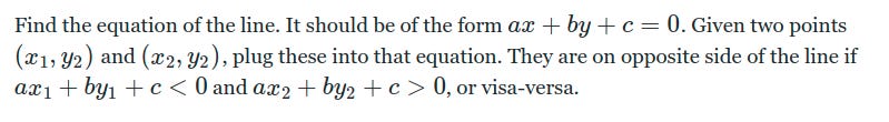
So I take the equation of the line, say “1x+1y+0”
Now consider 2 points (1,1) and (-6,-1)
For point (1, 1) => 1(1)+ 1(1) = 2 which is > 0
For point (-6, -1) = 1(-6)+(1)(-1) = -7 which is < 0
Therefore, we can conclude that (1,1) and (-6,-1) lie on different sides of the line S.
Now in the given problem, given an equation — all red should be on one side of the equation and blue on the other side.
General Mathematical Principle
Here’s the Algorithm I will follow for the below Python Implementation
The question already mentioned — “you need to do string parsing here and get the coefficients of x,y and intercept”
I know the string in the Equation will be of the form
some_number*xandsome_number*y, where the 'some_number' is the coefficients of x and y. So I need to break the string up in such a way that I am only left with just the numbers, and then replace the value of x and y in the equation with the value of the points that I am evaluating.Initiate a variable
sign_of_equation_with_red_point_tupleto be minus 1 (-1)Take the first tuple of the Red_side list (i.e. red[0][0] and red0 ) and replace then into the Equation. If sign of Equation becomes positive with this, then change
sign_of_equation_with_red_point_tupleto be plus 1 ( 1 )Now assuming
sign_of_equation_with_red_point_tupleto be plus one ( 1 ) do the below stepOne by one, check for all the Red side’s tuples (points) — if Equation sign becomes negative for any point > That means that single point is on the other side of the Line Equation.
So in that case, then return ‘NO’ from the function.
Similarly in the next step, assuming
sign_of_equation_with_red_point_tupleto be negaive 1 (-1), do the below stepOny by one, check for all the Red side’s tuples (points) — if Equation sign becomes positive for any point > That means that single point is on the other side of the Line Equation.
So in that case, then return ‘NO’ from the function.
Do both the above steps for the Blue side as well.
And if none of the above 4 steps returns a ‘NO’ ans, then finally return ‘YES’ from the function.
import math
def find_who(red, blue, line):
    sign_of_r_pts_eq = -1

    if eval(line.replace('x', '***%s**' % red[0][0]).replace('y', '***%s**' % red[0][1])) > 0:
        sign_of_r_pts_eq = 1

    for r_pt **in** red:
        if sign_of_r_pts_eq == 1 **and** eval(
                line.replace('x', '***%s**' % r_pt[0]).replace('y', '***%s**' % r_pt[1])) < 0:
            return 'NO'

        if sign_of_r_pts_eq == -1 **and** eval(
                line.replace('x', '***%s**' % r_pt[0]).replace('y', '***%s**' % r_pt[1])) > 0:
            return 'NO'


    sign_of_b_pts_eq = -1 * sign_of_r_pts_eq

    for b_pts **in** blue:
        if sign_of_b_pts_eq == 1 **and** eval(
                line.replace('x', '***%s**' % b_pts[0]).replace('y', '***%s**' % b_pts[1])) < 0:
            return 'NO'

        if sign_of_b_pts_eq == -1 **and** eval(
                line.replace('x', '***%s**' % b_pts[0]).replace('y', '***%s**' % b_pts[1])) > 0:
            return 'NO'

    return 'YES'


Red = [(1, 1), (2, 1), (4, 2), (2, 4), (-1, 4)]
Blue = [(-2, -1), (-1, -2), (-3, -2), (-3, -1), (1, -3)]

Lines = ["1x+1y+0", "1x-1y+0", "1x+0y-3", "0x+1y-0.5"]

for i **in** Lines:
    yes_or_no = find_who(Red, Blue, i)
    print(yes_or_no)

YES
NO
NO
YES
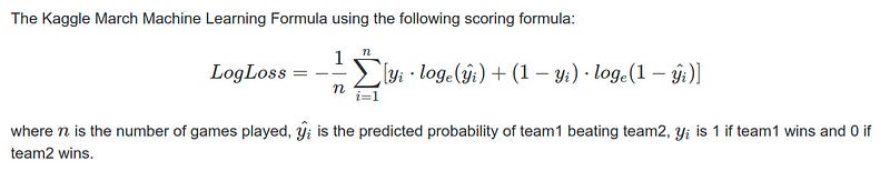
Q — Implement Log-Loss Function in Plain Python
You will be given a list of lists, each sublist will be of length 2 i.e. [[x,y],[p,q],[l,m]..[r,s]] consider its like a matrix of n rows and two columns
a. the first column Y will contain integer values
b. the second column 𝑌𝑠𝑐𝑜𝑟𝑒Yscore will be having float values
Your task is to find the value of the below
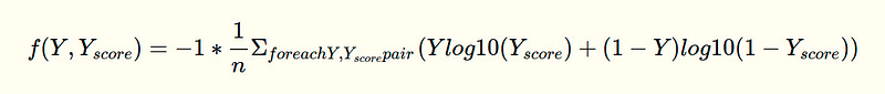
Ex: [[1, 0.4], [0, 0.5], [0, 0.9], [0, 0.3], [0, 0.6], [1, 0.1], [1, 0.9], [1, 0.8]] output: 0.4243099
Explanations and Notes on Log Loss
Logarithmic Loss (i.e. Log Loss and also same as Cross Entropy Loss), is a classification loss function. Log Loss quantifies the accuracy of a classifier by penalising false classifications. Minimising the Log Loss is basically equivalent to maximising the accuracy of the classifier.
Log loss is used when we have {0,1} response. In these cases, the best models give us values in terms of probabilities. The log loss function is simply the objective function to minimize, in order to fit a log linear probability model to a set of binary labeled examples.
In slightly different form Log is expressed as
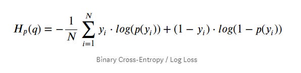
Log Loss is a slight modification on the Likelihood Function. In fact, Log Loss is -1 * the log of the likelihood function.
Log Loss measures the accuracy of a classifier. It is used when the model outputs a probability for each class, rather than just the most likely class.
In simple words, log loss measures the UNCERTAINTY of the probabilities of your model by comparing them to the true labels. Let us look closely at its formula and see how it measures the UNCERTAINTY.
Now the question is, your training labels are 0 and 1 but your training predictions are 0.4, 0.6, 0.89, 0.1122 etc.. So how do we calculate a measure of the error of our model ? If we directly classify all the observations having values > 0.5 into 1 then we are at a high risk of increasing the miss-classification. This is because it may so happen that many values having probabilities 0.4, 0.45, 0.49 can have a true value of 1.
This is where logLoss comes into picture.
Log-loss is a “soft” measurement of accuracy that incorporates the idea of probabilistic confidence. It is intimately tied to information theory: log-loss is the cross entropy between the distribution of the true labels and the predictions. Intuitively speaking, entropy measures the unpredictability of something. Cross entropy incorporate the entropy of the true distribution, plus the extra unpredictability when one assumes a different distribution than the true distribution. So log-loss is an information-theoretic measure to gauge the “extra noise” that comes from using a predictor as opposed to the true labels. By minimizing the cross entropy, one maximizes the accuracy of the classifier.
Cases where Log-Loss function can be mostly used
The log loss function is used as an evaluation metric of the ML classifier models. This is an important metric as it is only metric which uses the actual predicted probability for evaluating the model ( ROC — AUC uses the order of the values but not the actual values). This is very useful as this penalizes the model heavily if it is very confident in predicting the wrong class(please check the plot of -log(x)). We optimize our model to minimize the log loss. Hence this metric is very useful in cases where the cost of predicting wrong class is very high. Hence model tries to reduce the probabilities of belonging to wrong class and we can choose the higher threshold of probability to predict the class label. This metric can be used for both binary and multi class classifications. The value of log loss lies between 0 ( including) and infinity. This is the only disadvantage of log loss as it is not very interpretable. We know that the best case would be 0 value of log loss however we can not interpret other values of log loss. For some cases log loss of 1 can be good while for other it may not be good enough. One hack is that we can measure the log loss of random model and try to reduce log-loss of our actual model from this value as much as possible without increasing variance.
Please note that this metric can only be used if our model can predict the probability of each class. Hence for calculating the log loss for the models which don’t provide the probability score, probability calibration methods can be used on top of the base classifier to predict the probability score for each class.
A use-case of Logloss
Say, I am predicting Cancer from my ML Model. And Suppose you have 5 cases. 2 cases were cancer (y1 = y2 = 1) and 3 cases were benign (y3 = y4 = y5 = 0). Say your model predicted each model has 0.5 probability of cancer. In this case, what we have for log loss is…
−1/5∗(log(0.5)+log(0.5)+(1−0)∗log(1−0.5)+(1−0)∗log(1−0.5)+(1−0)∗log(1−0.5))
Essentially, y_i and (1 — y_i) determines which term is to be dropped depending on the ground truth label. Depending on ground truth, either the log (y_hat) or log(1-y_hat) will be selected to determines how far away from the truth your model’s generated probability is.
We can use the log_loss function from scikit-learn, with documentation found here: But here we will implement a pure-python version
Finally Simple Python Implementation
from math import log
def get_loss_log(matrix):
    logistic_loss = 0
    for row **in** matrix:
        logistic_loss += (row[0] * log(row[1], 10) + ((1 - row[0]) * log(1 - row[1], 10)))

    log_loss = -1 * logistic_loss / len(matrix)
    return log_loss


A = [[1, 0.4], [0, 0.5], [0, 0.9], [0, 0.3], [0, 0.6], [1, 0.1], [1, 0.9], [1, 0.8]]
print(get_loss_log(A))
Gradient Descent in Python from scratch without using any library
import numpy as np
import random
import pandas as pd


'''
  Gradient Descent for a single feature
  It will NOT work for multiple feature
'''

number_of_data_points = 50

# For predictor x, generate a Numpy array containing number betwen 2 and 9
x = np.random.randint(2, 9, number_of_data_points)

# print('x before dataframe ', x)
x = pd.DataFrame(x)
# print('df ', x)

# Standardize x
x = (x - x.mean()) / x.std()

# ***************************************************************

# Add one column for gradient-descent
x = np.c_[np.ones(x.shape[0]), x]
# print('x after adding one column ', x)

# For the target variable y, generate a Numpy array containing number betwen 1 and 26
y = np.random.randint(1, 26, number_of_data_points )
y = pd.DataFrame(y, columns = ['Y-Value'])
y = y['Y-Value']

# ********* Now the Gradient descent formulae implementation **********

alpha = 0.01 # Learning Step size
iterations = 100 #No. of iterations
np.random.seed(123) #Set the seed
theta = np.random.rand(2) #Pick some random values to start with


### GRADIENT DESCENT

def gradient_descent(x, y, theta, iterations, alpha):
    prev_cost = []
    prev_thetas = [theta]
    for i in range(iterations):
        prediction = np.dot(x, theta)
        error = prediction - y

        cost = 1/(2*number_of_data_points) * np.dot(error.T, error)
        prev_cost.append(cost)
        theta = theta - (alpha * (1/number_of_data_points) * np.dot(x.T, error))
        prev_thetas.append(theta)

    return prev_thetas, prev_cost


prev_thetas, prev_cost = gradient_descent(x, y, theta, iterations, alpha)
theta = prev_thetas[-1]

print("Gradient Descent: {:.2f}, {:.2f}".format(theta[0], theta[1]))