
RNNs just got a nitro boost: FlashRNN makes GPUs go zoom.
50x speedup over vanilla PyTorch implementation. This Revolutionary State Tracking Could Save 60% of AI Processing Costs

Paper - https://arxiv.org/abs/2412.07752
Github - https://github.com/NX-AI/flashrnn
Traditional RNNs are powerful for tasks that require state tracking, such as time-series forecasting and logical sequence tasks, but they are inherently limited by their strictly sequential computation—each time step depends on the output of the previous one.
 — A Gateway to Sequential Data Analysis | by Palash Mishra | Medium")
This sequential nature makes them much slower than architectures like Transformers, which parallelize computations across the entire sequence. Despite their potential, standard RNN implementations fail to fully utilize modern GPU hardware. GPUs are designed for massive parallelism and have a complex memory hierarchy, ranging from ultra-fast registers to shared memory (SRAM) and global high-bandwidth memory (HBM).
However, vanilla RNNs often over-rely on HBM for every time step, leading to bottlenecks due to frequent memory access. Additionally, the lack of register-level optimizations—where computations stay closer to the GPU’s arithmetic units—means that RNNs miss out on the speed boosts that GPUs could provide if memory-intensive operations were minimized.
This inefficiency makes RNNs impractical for large-scale sequence modeling compared to the highly parallelizable and GPU-friendly design of Transformers. FlashRNN addresses this issue by rethinking how memory and computation are handled in RNNs, closing the performance gap with specialized optimizations.
FlashRNN introduces a way to optimize traditional Recurrent Neural Networks (RNNs) like LSTMs (Long Short-Term Memory) and GRUs (Gated Recurrent Units) for modern GPUs by improving how computations are parallelized and how memory is managed. Despite the hype around Transformers, RNNs remain unbeatable in state-tracking tasks like time-series predictions and logic-related tasks. The challenge is their strict sequential processing, which makes them slow. FlashRNN aims to fix this without changing the core RNN design.
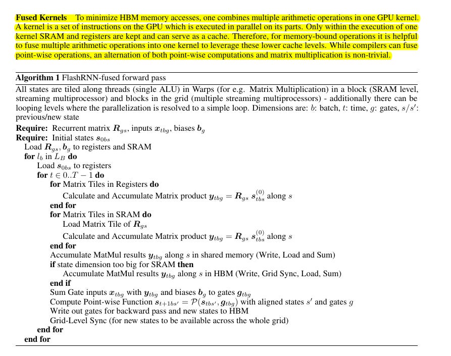
The core idea is to fuse operations into a single GPU kernel. In vanilla RNNs, each time step runs separately, with matrix multiplications and non-linear activations alternating between each step. This constant back-and-forth access to memory slows things down. FlashRNN combines these operations into one "fused kernel," which minimizes memory reads/writes and uses faster on-chip memory like registers and shared memory (SRAM) rather than the slower GPU high-bandwidth memory (HBM).
Fused kernel
→ What is a Kernel on a GPU?
A kernel is a set of GPU instructions that run in parallel. These instructions could be anything from matrix multiplications to pointwise activations (like sigmoid or tanh). Typically, each kernel processes a small piece of data at a time, reading from and writing to GPU memory.
→ Why Fused Kernels?
Each time the GPU reads from or writes to high-bandwidth memory (HBM), it incurs a significant latency cost. Instead of launching multiple kernels for different tasks—like computing a matrix product, summing it, and applying an activation function—a fused kernel combines all these tasks into a single operation. This reduces the number of memory accesses by keeping intermediate results in faster memory, such as registers and shared memory (SRAM), rather than repeatedly accessing HBM.
→ How Fused Kernels Work in FlashRNN
FlashRNN optimizes the forward pass of RNNs using fused kernels, which combine key operations across time steps in a single GPU pass:
Loading into Fast Memory: The recurrent states (R) and biases (b) are loaded into registers and shared memory for quick access.
Matrix Multiplication in Registers: Instead of writing intermediate matrix multiplication results to HBM, they are kept directly in registers.
Pointwise Operations in a Single Flow: Activation functions (non-linear operations like ReLU, sigmoid) are applied immediately within the same kernel, avoiding a second read/write step.
Accumulation: Outputs are summed across shared memory levels and only stored back to HBM at the end of the full computation loop.
Breaking Down the FlashRNN Kernel
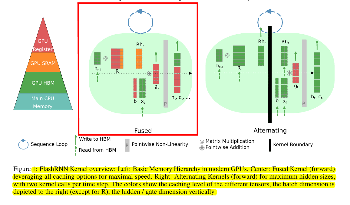
This image from the presents a breakdown of GPU memory hierarchy and the concept of fused versus alternating kernels in the FlashRNN model, highlighting how different approaches to computation and memory usage can impact performance.
The "fused kernel" for the forward pass processes the input sequence in a loop, step-by-step through time. Instead of alternating between separate operations for matrix multiplication and activations, everything is packed into one kernel.
→ Memory Hierarchy (Left Panel):
The pyramid shows memory levels in decreasing order of speed and increasing capacity.
Registers (at the top): Fastest but smallest memory used for immediate operations.
SRAM (Shared Memory): On-chip, faster than high-bandwidth memory (HBM), useful for temporary data sharing between threads.
HBM (High-Bandwidth Memory): Slower external GPU memory, typically used for reading and writing larger data chunks.
CPU Memory: Slowest and farthest from the GPU cores, often used for large datasets that won’t fit on the GPU.
→ Fused Kernel (Center Panel):
A fused kernel combines multiple operations—like matrix multiplications, additions, and nonlinearities—into one pass.
Instead of writing intermediate outputs back to the slower HBM after each step, it keeps everything in the faster on-chip memory (registers and SRAM) as much as possible.
In this diagram, you can see that only the final output (hidden states and cell states) is written back to the HBM once per sequence step, minimizing memory traffic.
→ Alternating Kernel (Right Panel):
The alternating approach splits the computations across multiple smaller kernels. This results in multiple memory read/write steps at the kernel boundaries (shown as vertical black lines).
Since the computation is broken into more stages, there are more frequent trips to slower HBM, increasing latency.
Here’s a simplified breakdown of the forward pass:
Initialization:
Load the recurrent weight matrix RRR, biases bbb, and initial states into faster GPU memory (registers and SRAM).
Matrix Multiplication:
Compute the gate preactivations gtg_tgt using tiled matrix multiplications, accumulating partial results in shared memory.
Memory Sync and Accumulation:
Combine results across different thread blocks if needed. This ensures all time-step computations are aligned.
Gate Computations:
Add bias terms and apply the point-wise functions (like sigmoid and tanh) to compute the next states st+1s_{t+1}st+1.
Final Write-Back:
Write the new hidden and cell states back to high-bandwidth memory (HBM) for backward pass storage.
Key Implementation Details
FlashRNN uses block-diagonal matrices to mimic how multi-head attention works in Transformers. Instead of handling a massive recurrent weight matrix as one big block, it divides it into smaller "heads." Each head processes smaller chunks of the hidden states independently. This means that even though RNNs can't be parallelized over time like Transformers, they can still parallelize over these smaller chunks.
The hardware-aware design optimizes memory hierarchies. Modern GPUs have registers (tiny but ultra-fast memory), SRAM (shared memory per compute unit), and HBM (global memory shared across all GPU cores). FlashRNN prioritizes keeping the recurrent matrix weights and biases in registers whenever possible. If the weights don’t fit, they move to SRAM. Only as a last resort are HBM accesses used.
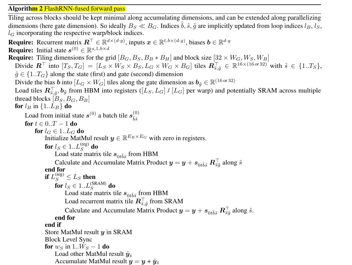
Tiling and Parallelism Explained
FlashRNN handles parallelism through "tiling." Tiling breaks the input data into smaller sub-blocks that fit into fast memory. It then processes these sub-blocks in parallel. For example, the recurrent weight matrix is sliced into "tiles" of smaller sizes that fit perfectly into registers. Each thread in a GPU block processes one tile, and multiple blocks handle different parts of the input sequence.
Since GPUs work best when computations are done in parallel, FlashRNN ensures that tiling happens along dimensions that don’t require sequential operations. For example, the "gate dimension" (which holds values for forget gates, input gates, etc.) is split across multiple threads, while the "time dimension" (which requires steps to happen in order) is processed sequentially.
Constraints and Tuning with ConstrINT
FlashRNN’s implementation adapts itself to different GPU hardware using an integer constraint solver called ConstrINT. This tool helps figure out how to set key parameters like the number of threads per block, the amount of data to load per loop, and the tiling sizes. ConstrINT takes into account things like the total size of registers, SRAM, and how many threads can run in parallel without memory conflicts.
The constraints are modeled as inequalities. For example, if a GPU has 256KB of shared memory and a recurrent matrix takes 4MB, the matrix must be split into smaller chunks that fit within the 256KB limit. ConstrINT automates this splitting while ensuring that performance isn’t compromised.
Results and Speedups
FlashRNN shows massive speed improvements—up to 50x faster than vanilla PyTorch LSTM implementations. The fused kernels also handle much larger hidden sizes (up to 40x larger) because of the efficient use of memory and parallelism. For small batch sizes, the "fused kernel" performs up to 3x faster than the alternating kernels, where each operation runs separately.
The performance gains come from reducing how often the GPU reads and writes from slow memory. Instead of fetching weights from HBM for every time step, FlashRNN keeps as much data as possible in registers, where access times are practically instant.
Overall, FlashRNN bridges the gap between state-tracking RNNs and the parallelizable world of GPUs. By fusing operations and using head-wise parallelism, it turns the sequential nature of RNNs into something that can efficiently utilize modern hardware. This approach opens new possibilities for faster sequence models that don’t need to sacrifice state-tracking capabilities.