
Table of Contents
Draft and Verify Decoding
Batched Speculative Decoding
Fast Forwarding with Smaller Draft Models
Budget Conscious Implementation Strategies
Startup vs Large Scale Deployment
Draft and Verify Decoding
Speculative decoding uses a draft-and-verify paradigm: a small “draft” model first proposes several tokens, then the large target model verifies those tokens in parallel. This allows multiple tokens to be generated per iteration instead of the usual one, substantially accelerating inference. In essence, the draft model guesses the next few tokens, and the main model checks these guesses in one forward pass, accepting the tokens that match its own distribution and correcting the first token that does not. The process is constructed to be lossless, i.e. it yields the same distribution of outputs as standard autoregressive decoding. This method trades some extra computation on the small model for far fewer sequential calls to the large model, often yielding 2× or more speedup in practice (BASS: Batched Attention-optimized Speculative Sampling).
How it works: At each step, the draft model generates a batch of candidate tokens one-by-one (like a tentative continuation). Then the main model is invoked once to score all those draft tokens at once. The main model’s output probabilities are compared against the draft tokens: it will accept a token if it agrees, or reject at the first point of disagreement. In case of a rejection, the main model’s chosen token at that position is used instead, and the verification step ends. Any remaining draft tokens after a rejection are discarded, and the process repeats. This draft-then-verify cycle continues until an end-of-sequence token or length limit is reached. For example, a draft model might propose the next five tokens "I", "like", "cooking", "and", "traveling" for a given context. The large model verifies them in one go; if it finds that the third token should be "playing" instead of "cooking", it would accept "I like", reject at the third token and replace it with "playing", then discard the remaining draft tokens. The verified sequence now continues from "I like playing". In the next iteration, the draft model will propose further tokens after "I like playing" and so on.
Why it’s beneficial: Verifying multiple tokens in parallel keeps the GPU busy with larger matrix multiplies (leveraging its full parallelism) instead of idle between token steps. The main model does more work per call but calls are fewer. The small model is much faster (due to far fewer parameters), so its token-by-token drafting is relatively cheap. The net effect is that overall latency is reduced – memory bandwidth is better utilized and total compute can drop. Empirical results in 2024 confirm significant gains: e.g. speculative decoding achieved a ~2.3× speedup in a vision-language model without quality loss, and 2×–3× speedups on text models are reported in multiple studies ( Medusa: Simple LLM Inference Acceleration Framework with Multiple Decoding Heads). A key requirement is that the draft and main model share the same vocabulary and are reasonably well-aligned in their predictions, to avoid frequent rejections (Training Domain Draft Models for Speculative Decoding: Best Practices and Insights). When those conditions hold, this method can drastically reduce end-to-end generation time while guaranteeing the same output distribution as the original model.
Below is a PyTorch implementation of basic draft-and-verify decoding. We define a dummy large model (main_model) and a dummy small model (draft_model) for illustration. The code generates text from main_model using draft_model to propose speculative tokens:
import torch
import torch.nn as nn
import torch.nn.functional as F

# Dummy language model definition (LSTM-based for sequential token prediction)
class DummyLM(nn.Module):
    def __init__(self, vocab_size, embed_dim, hidden_dim):
        super().__init__()
        self.embed = nn.Embedding(vocab_size, embed_dim)
        self.lstm = nn.LSTM(embed_dim, hidden_dim, batch_first=True)
        self.linear = nn.Linear(hidden_dim, vocab_size)
    def forward(self, input_ids):
        # input_ids: Tensor of shape (1, seq_len)
        embeds = self.embed(input_ids)
        outputs, _ = self.lstm(embeds)
        logits = self.linear(outputs)  # shape (1, seq_len, vocab_size)
        return logits

# Instantiate a large model and a smaller draft model
vocab_size = 1000
main_model = DummyLM(vocab_size, embed_dim=64, hidden_dim=128)
draft_model = DummyLM(vocab_size, embed_dim=64, hidden_dim=64)

# Example initial context (prompt) and generation parameters
context_tokens = 1, 5, 42  # some tokenized input prompt
max_new_tokens = 20
draft_length = 4  # number of speculative tokens to draft per iteration

# Move models to eval mode
main_model.eval(); draft_model.eval()

# Start speculative decoding
generated = context_tokens.copy()
for _ in range(max_new_tokens):
    # 1. Draft phase: use small model to propose `draft_length` tokens
    draft_tokens =
    ctx = torch.tensor(generated).unsqueeze(0)  # shape (1, current_length)
    for i in range(draft_length):
        with torch.no_grad():
            logits = draft_model(ctx)               # draft model predictions for each position
            next_token_logits = logits0, -1, :    # logits for the next token
        # choose the draft token (greedy for simplicity; could sample for true distribution matching)
        draft_token = int(torch.argmax(next_token_logits))
        draft_tokens.append(draft_token)
        # append draft token to context for next iteration of draft model
        ctx = torch.cat(ctx, torch.tensor(), dim=1)
        # optional: break if EOS token is generated
        if draft_token == 0:  # assume 0 is EOS token for illustration
            break

    # 2. Verify phase: use main model to verify the draft in one forward pass
    with torch.no_grad():
        # prepare input: existing generated sequence + draft tokens
        input_ids = torch.tensor(generated + draft_tokens).unsqueeze(0)
        logits_seq = main_model(input_ids)  # shape: (1, len(generated)+len(draft_tokens), vocab_size)
    # Extract the logits corresponding to each drafted token position
    start_idx = len(generated)  # index where draft tokens start in the sequence
    verified_count = 0
    for j, draft_token in enumerate(draft_tokens):
        main_pred_logits = logits_seq0, start_idx + j, :      # main model's prediction at this position
        main_pred_token = int(torch.argmax(main_pred_logits))   # token the main model would produce
        if main_pred_token == draft_token:
            # Accept the draft token since main model agrees
            generated.append(draft_token)
            verified_count += 1
            if draft_token == 0:  # EOS from draft (and accepted by main)
                break  # stop generation
        else:
            # Reject at the first mismatch:
            generated.append(main_pred_token)  # use main model's token instead
            # (Discard the rest of draft_tokens beyond this point)
            break
    if verified_count == len(draft_tokens):
        # All draft tokens were accepted; we have effectively fast-forwarded by `draft_length` tokens
        continue  # continue to next iteration without adding a new main token this round
    # If a rejection happened or EOS encountered, we end this iteration (a new main token was added or sequence ended)
    if generated-1 == 0 or len(generated) >= len(context_tokens) + max_new_tokens:
        break

print("Generated sequence:", generated)
In this code, draft_model proposes up to draft_length tokens beyond the current generated sequence. The main_model then produces logits for each position of these new tokens in one batch (logits_seq). We compare each draft token against the main_model’s predicted token. The loop breaks at the first disagreement, where the main model’s token is used instead of the draft’s. All tokens before that point are accepted, effectively skipping those individual decoding steps. If the draft tokens are all accepted (no mismatch), the loop continues, having fast-forwarded the generation by several tokens in one go. The process repeats until the sequence is complete. In a real implementation, the acceptance criterion can be more nuanced (e.g. based on probability ratios to ensure exact distributional equivalence), and typically both models would sample from their probability distributions (not always take argmax) to avoid bias. Here we use a simplified greedy approach for clarity.
Where it fits in the pipeline: This draft-and-verify procedure replaces the standard token-by-token generation loop in the decoder. Instead of calling the large model for each new token, we call the large model less frequently – only after drafting a batch of tokens. This dramatically reduces the number of sequential decoder calls. In practice, one would load both the large and small model in memory. On each iteration, the small model runs on the given context to propose tokens, then the large model runs to validate them. Modern inference frameworks have built-in support for this pattern; e.g., vLLM introduces separate “draft” and “target” runners that orchestrate the two models and manage their key-value caches for attention. The result is that each cycle processes multiple tokens and keeps the GPU utilization high, rather than doing many tiny one-token steps. The overall latency improvement is significant especially for long sequences or large models, where the overhead of many sequential passes is highest.
Batched Speculative Decoding
Scaling to multiple sequences: The standard speculative decoding above focuses on one sequence at a time. However, real-world deployments often need to generate many sequences concurrently (e.g. multiple user queries in a batch). Naively, one might try to run draft-and-verify for a batch of requests together, but this introduces challenges. If we force all sequences in a batch to use the same number of draft tokens per step, a single sequence’s rejection could invalidate draft tokens for others, wasting computation (BASS: Batched Attention-optimized Speculative Sampling). In fact, with batch size > 1, the chance that all sequences accept a given draft token is the product of individual acceptance rates, which drops quickly as batch size grows . For example, if each token has a 20% chance of being accepted for one sequence, that sequence advances ~5 tokens per speculative iteration on average. But in a batch of 5 simultaneous sequences, the probability all 5 accept a token is only 0.2^5 = 0.032 (3.2%), dramatically reducing the average progress per iteration to ~1.5 tokens . In other words, a synchronous draft for the whole batch would squander most of the speedup, since one sequence’s early rejection forces others to stop verification early . The key to batched speculative decoding is allowing each sequence to accept a variable number of draft tokens independently, within the same parallel step.
Batched strategy: Recent work addresses this with dynamic batching and scheduling techniques. BASS (Batched Attention-optimized Speculative Sampling) generalizes speculative decoding to the batch setting by using specialized tensor operations to accommodate different draft lengths per sequence within one joint forward pass . Essentially, each sequence can draft a different number of tokens, and the main model verifies all sequences in one go by padding shorter drafts and masking out unused positions. The implementation requires careful low-level kernel optimization to avoid wasting computation on padded tokens and to handle divergent control flow when different sequences reject at different points . The result is that we can achieve high parallelism across both tokens and sequences. This maximizes GPU utilization and throughput, especially on modern hardware where large batch matrix multiplies are most efficient.
Performance: Batched speculative decoding can lead to superlinear speedups in multi-request settings. By combining inter-sequence batching with intra-sequence speculative leaps, the throughput scales very favorably. For example, with a 7.8B model on a single A100 GPU and batch size 8, BASS achieved ~5.8 ms per token per sequence (over 1.1k tokens/sec total throughput), a 2.15× speed-up over optimized single-sample decoding. Importantly, within a fixed time budget, the batched spec decoding system can generate much more text (and of higher quality) than either standard decoding or one-sequence-at-a-time speculative decoding. GPU utilization in such scenarios reached ~15.8% (still low in absolute terms, but over 3× higher than regular decoding and ~10× higher than naive single-sequence speculative decoding). This indicates the approach effectively alleviates the memory bandwidth bottleneck by keeping more of the hardware busy with useful work across the batch.
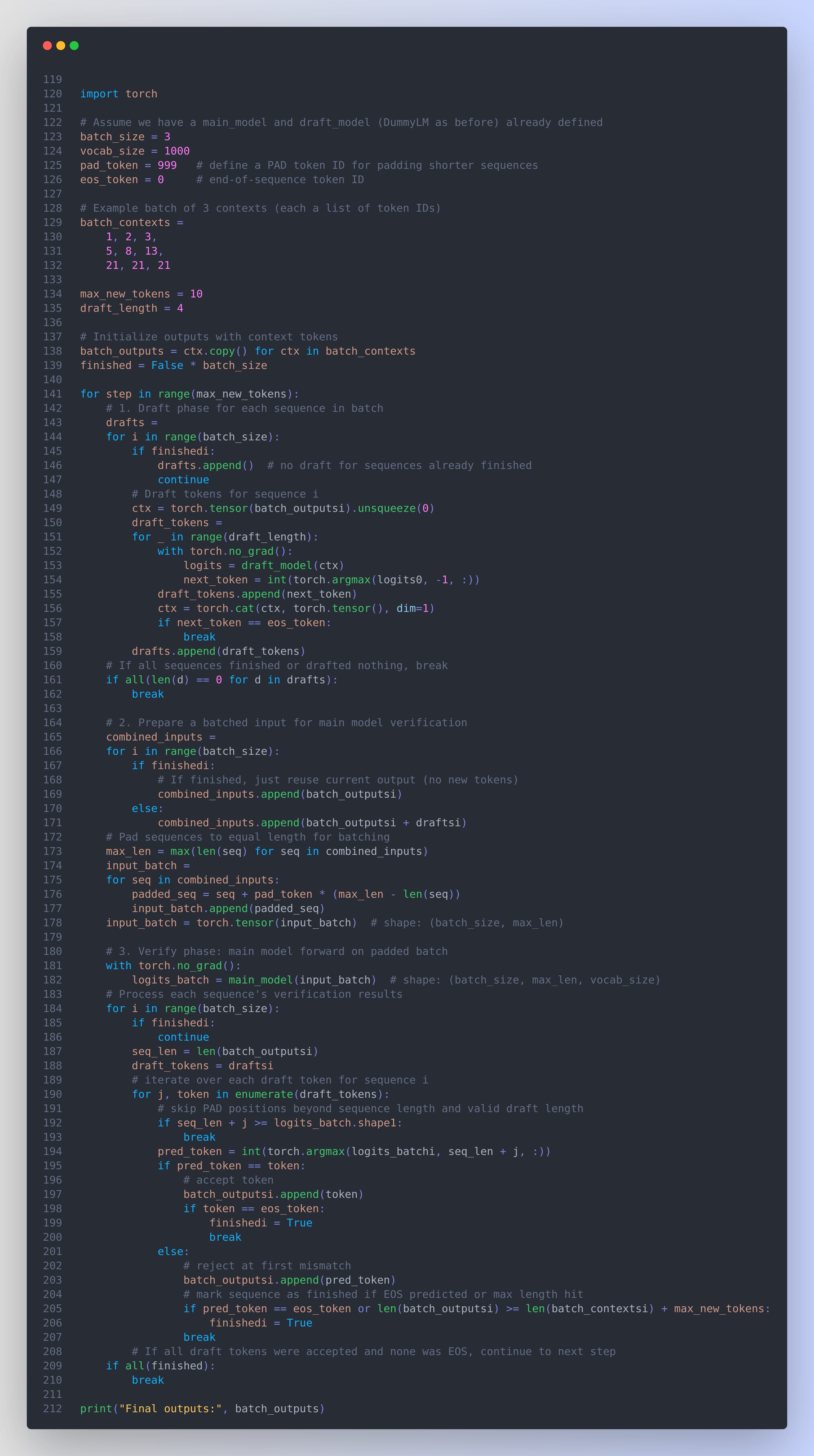
Implementation approach: To illustrate batched speculative decoding, consider the following PyTorch code that extends the draft-and-verify example to multiple sequences. We simulate how different sequences in a batch can accept different numbers of draft tokens, and how to manage padding for a joint verification by the main model:
import torch

# Assume we have a main_model and draft_model (DummyLM as before) already defined
batch_size = 3
vocab_size = 1000
pad_token = 999   # define a PAD token ID for padding shorter sequences
eos_token = 0     # end-of-sequence token ID

# Example batch of 3 contexts (each a list of token IDs)
batch_contexts =
    1, 2, 3,
    5, 8, 13,
    21, 21, 21

max_new_tokens = 10
draft_length = 4

# Initialize outputs with context tokens
batch_outputs = ctx.copy() for ctx in batch_contexts
finished = False * batch_size

for step in range(max_new_tokens):
    # 1. Draft phase for each sequence in batch
    drafts =
    for i in range(batch_size):
        if finishedi:
            drafts.append()  # no draft for sequences already finished
            continue
        # Draft tokens for sequence i
        ctx = torch.tensor(batch_outputsi).unsqueeze(0)
        draft_tokens =
        for _ in range(draft_length):
            with torch.no_grad():
                logits = draft_model(ctx)
                next_token = int(torch.argmax(logits0, -1, :))
            draft_tokens.append(next_token)
            ctx = torch.cat(ctx, torch.tensor(), dim=1)
            if next_token == eos_token:
                break
        drafts.append(draft_tokens)
    # If all sequences finished or drafted nothing, break
    if all(len(d) == 0 for d in drafts):
        break

    # 2. Prepare a batched input for main model verification
    combined_inputs =
    for i in range(batch_size):
        if finishedi:
            # If finished, just reuse current output (no new tokens)
            combined_inputs.append(batch_outputsi)
        else:
            combined_inputs.append(batch_outputsi + draftsi)
    # Pad sequences to equal length for batching
    max_len = max(len(seq) for seq in combined_inputs)
    input_batch =
    for seq in combined_inputs:
        padded_seq = seq + pad_token * (max_len - len(seq))
        input_batch.append(padded_seq)
    input_batch = torch.tensor(input_batch)  # shape: (batch_size, max_len)

    # 3. Verify phase: main model forward on padded batch
    with torch.no_grad():
        logits_batch = main_model(input_batch)  # shape: (batch_size, max_len, vocab_size)
    # Process each sequence's verification results
    for i in range(batch_size):
        if finishedi:
            continue
        seq_len = len(batch_outputsi)
        draft_tokens = draftsi
        # iterate over each draft token for sequence i
        for j, token in enumerate(draft_tokens):
            # skip PAD positions beyond sequence length and valid draft length
            if seq_len + j >= logits_batch.shape1:
                break
            pred_token = int(torch.argmax(logits_batchi, seq_len + j, :))
            if pred_token == token:
                # accept token
                batch_outputsi.append(token)
                if token == eos_token:
                    finishedi = True
                    break
            else:
                # reject at first mismatch
                batch_outputsi.append(pred_token)
                # mark sequence as finished if EOS predicted or max length hit
                if pred_token == eos_token or len(batch_outputsi) >= len(batch_contextsi) + max_new_tokens:
                    finishedi = True
                break
        # If all draft tokens were accepted and none was EOS, continue to next step
    if all(finished):
        break

print("Final outputs:", batch_outputs)
This code processes a batch of sequences together. Each sequence i gets its own speculative draft_tokens list. We then concatenate each context with its drafts and pad all sequences to the same length (max_len) so they can be fed through main_model in one go as a batch tensor. The main model’s logits for each sequence are then checked token-by-token. Each sequence can accept a different number of draft tokens (some may break at an early mismatch, others may accept all). We mark sequences as finished if an end-of-sequence token is produced or if they hit the length limit. Notably, padding ensures that shorter sequences (or those that hit a rejection early) do not interfere with longer ones in the batch; the main model still computed logits for padded positions, but those are ignored. In an optimized system, one would avoid computing needless positions via custom kernels or masking, to save work (BASS: Batched Attention-optimized Speculative Sampling). The above code prioritizes clarity: it loops over sequences for the draft and verification steps. A real implementation would vectorize operations where possible (e.g., combine the draft model calls using one padded batch as well).
Where it fits in the pipeline: Batched speculative decoding is a serving-time optimization that sits at the request batching layer. In a production environment, one typically groups incoming requests or multiple generation tasks into batches to maximize GPU utilization. With this method, the scheduler can still batch requests together, but it must handle that each sequence might advance by a different number of tokens per iteration. Systems like vLLM already perform continuous batching, packing multiple requests into one forward pass; integrating speculative decoding means the scheduler now batches multiple tokens per request as well. The interaction between the “draft runner” and “target runner” becomes more complex: after each target verification pass, sequences in the batch will have progressed by varying amounts. The scheduler can then assemble the next batch of draft proposals accordingly (some sequences might have ended or be waiting for fewer tokens). In large-scale deployments, this requires careful book-keeping and dynamic tensor slicing. The reward is higher throughput and better latency scaling with batch size. Put simply, batched speculative decoding pushes utilization toward the limit by ensuring both token-level parallelism (via drafting multiple tokens) and sequence-level parallelism (via batching multiple sequences) are exploited.
Fast Forwarding with Smaller Draft Models
The draft-and-verify approach can be extended and optimized in various ways using smaller models to “fast-forward” the generation. The goal of these methods is to push even more work onto cheaper computation (small models or extra prediction heads) so that the large model’s workload is minimized. We highlight three notable strategies: integrating multi-token predictors into the large model, using advanced draft models with lookahead capabilities, and leveraging hierarchical or multiple draft models.
(a) Integrated multi-token predictors (Medusa): One limitation of basic speculative decoding is the need for a separate draft model that shares the vocabulary and is well-aligned with the large model. Medusa (Cai et al., 2024) eliminates the external model by adding lightweight multiple decoding heads to the large model itself ( Medusa: Simple LLM Inference Acceleration Framework with Multiple Decoding Heads). Each head is trained to predict tokens further ahead in the sequence (for example, head 1 predicts the next token, head 2 predicts the token after that, etc.), enabling the model to propose a tree of possible continuations internally. In each step, Medusa’s heads generate multiple candidate next-token sequences in parallel, and a modified attention mechanism in the model verifies these candidates simultaneously . Essentially, the large model “branches out” several steps and checks its own branches in one go. This can drastically reduce the number of sequential steps required. Medusa offers two modes: Medusa-1, where only the new heads are fine-tuned on a frozen large model (preserving original model output exactly, a lossless speedup), and Medusa-2, where the whole model and heads are fine-tuned together for even better prediction accuracy (allowing greater speedups at the cost of requiring careful training) . Reported speedups are 2.2× (lossless) up to 3.6× with slight trade-offs . The challenge, however, is the extra training complexity and the need to maintain multiple prediction heads. As noted by the ReDrafter authors, Medusa’s independent multi-head predictions do not leverage the sequential dependency structure and can explode the space of candidates exponentially, which may limit accuracy beyond a few tokens of lookahead. Still, Medusa demonstrates an effective way to fast-forward by augmenting the large model itself with speculative capabilities instead of using an external draft model.
(b) Advanced draft models (Recurrent draft and beam search): Another strategy is to design a more powerful draft model that can predict longer sequences with higher fidelity to the large model. If the draft model can reliably propose a long stretch of correct tokens, the big model can accept more and skip farther ahead. ReDrafter (Cheng et al., 2024) exemplifies this approach: it uses a recurrent neural network (RNN) as the draft model that conditions on the large model’s hidden state to generate a sequence of tokens. At each step, ReDrafter actually lets the large model output the first token (to ground the process), then feeds the large model’s last-layer hidden state into a small RNN which continues generating subsequent tokens (possibly using beam search to consider multiple candidate continuations). The large model then verifies the RNN’s proposed continuation; if there’s a mismatch, only the first token was guaranteed by the large model anyway (so output quality remains exact). By integrating the draft process with the large model’s internal state, the draft model has much better guidance and can predict more accurately than an uninformed external model. ReDrafter also applies knowledge distillation from the large model to the draft RNN during training, ensuring the RNN’s predictions align closely with the large model’s distribution. Through these techniques, ReDrafter achieves state-of-the-art speedups (~2.8× faster inference on GPU for Vicuna models, and up to 2.3× on an Apple M2 GPU) without any loss in output quality. An added benefit observed is that this method effectively mitigates memory bottlenecks: on slower hardware where the large model is memory-bound, speculative draft generation keeps the compute units fed with work. The complexity here is that one must train and maintain a custom draft model (the RNN) and possibly a beam search procedure for generation. But it demonstrates that smarter draft models = fewer large-model calls.
(c) Hierarchical or multi-model speculation: Instead of one draft model, some approaches cascade multiple draft models or multiple draft attempts to further accelerate generation. For example, the SPIN system (Chen et al., 2025) uses heterogeneous speculative models of different sizes and a selection algorithm to handle requests of varying difficulty. A simpler request might use a very small draft model, whereas a complex request uses a larger draft model – this adaptive strategy keeps the acceptance rate high without overpaying for an unnecessarily large draft on easy prompts. Other research explores draft-model-free speculation, where heuristics or cached patterns generate token guesses without a learned model. For instance, “prompt lookup” methods cache common n-gram continuations and use those as speculative drafts. Another line is tree-based speculative search (e.g. EAGLE and EAGLE-2): the draft model generates a tree of possible future tokens (branching out multiple tokens at each depth), and the large model then traverses this tree to find the longest acceptable path. EAGLE-2 improved this by dynamically adjusting the draft tree depth based on context, achieving speedups over 3× while ensuring the output distribution remains exactly the same as the original model (a provably lossless speedup). These approaches effectively fast-forward the decoding by exploring multiple future possibilities in parallel and only rarely falling back to step-by-step decoding. They tend to be more complex to implement and may require careful calibration of acceptance thresholds and model confidence, but they represent the frontier of maximizing inference efficiency.
To illustrate a fast-forward approach with code, below we implement a hybrid draft model that integrates with the large model’s hidden state. We simulate an idea similar to ReDrafter: after generating one token with the main model, we use a small RNN to quickly generate additional tokens before the next main model call:
import torch
import torch.nn as nn

# Assuming main_model is a DummyLM as defined earlier (with an LSTM),
# we will get its hidden state and use a small RNN to generate multiple tokens.
# Define a small RNN draft model (single-step GRU cell for simplicity)
input_dim = 128  # assume main_model hidden state size is 128
draft_hidden_dim = 64
draft_vocab_size = 1000

small_rnn = nn.GRUCell(input_dim, draft_hidden_dim)
small_out = nn.Linear(draft_hidden_dim, draft_vocab_size)
# (In practice, we would also have an embedding for input tokens to the GRU,
# but here we'll feed main model's hidden state directly.)

# Start with some context
context = 7, 7, 7  # example prompt
generated = context.copy()
max_steps = 10
draft_steps = 3

# We'll manually run main_model to get hidden state (since DummyLM.forward returns logits,
# we can modify DummyLM to also output hidden state, or reconstruct via its LSTM)
# For demonstration, run the LSTM portion directly to get hidden state after context.
context_tensor = torch.tensor(context).unsqueeze(0)
embeds = main_model.embed(context_tensor)
output, (h_n, c_n) = main_model.lstm(embeds)  # h_n is hidden state of shape (1, batch, hidden_dim)
main_hidden = h_n-1, 0, :  # last layer's hidden for last token

for step in range(max_steps):
    # Large model generates one token (we use the last hidden state and final layer for simplicity)
    # Normally, you'd feed the last token through the model to get next token.
    logits = main_model.linear(main_hidden.unsqueeze(0))  # project hidden to vocab
    main_token = int(torch.argmax(logits0, :))
    generated.append(main_token)
    if main_token == eos_token or len(generated) >= len(context)+max_steps:
        break  # stop if end-of-sequence or length reached

    # Use small RNN (draft model) to generate multiple tokens conditioned on main_hidden
    draft_tokens =
    # Initialize draft RNN hidden state as a transformation of main_hidden
    draft_h = torch.tanh(nn.Linear(input_dim, draft_hidden_dim)(main_hidden))
    prev_token_embed = torch.zeros(input_dim)  # no previous token, we use zero as start (could use embed of main_token)
    for _ in range(draft_steps):
        # One GRU step
        draft_h = small_rnn(prev_token_embed, draft_h)
        draft_logits = small_out(draft_h)
        next_token = int(torch.argmax(draft_logits))
        if next_token == eos_token:
            draft_tokens.append(next_token)
            break
        draft_tokens.append(next_token)
        # Update prev_token_embed for next iteration (use main_model's embedding for consistency)
        prev_token_embed = main_model.embed(torch.tensor(next_token))
    # Verify draft_tokens with main_model in one go
    verify_input = torch.tensor(generated + draft_tokens).unsqueeze(0)
    logits_seq = main_model(verify_input)
    base_idx = len(generated)  # index where draft starts
    for j, token in enumerate(draft_tokens):
        pred = int(torch.argmax(logits_seq0, base_idx + j, :))
        if pred == token:
            generated.append(token)  # accept token
            # If needed, update main_hidden by running this token through LSTM:
            # (Simplified: treat pred as accepted, we would update main_hidden via LSTM step if continuing loop)
        else:
            generated.append(pred)   # use main model token instead
            break
    # Update main_hidden for next iteration (recompute from new last token):
    last_token_id = generated-1
    last_token_embed = main_model.embed(torch.tensor())
    _, (h_n, c_n) = main_model.lstm(last_token_embed, (h_n, c_n))
    main_hidden = h_n-1, 0, :
    if generated-1 == eos_token:
        break

print("Generated sequence:", generated)
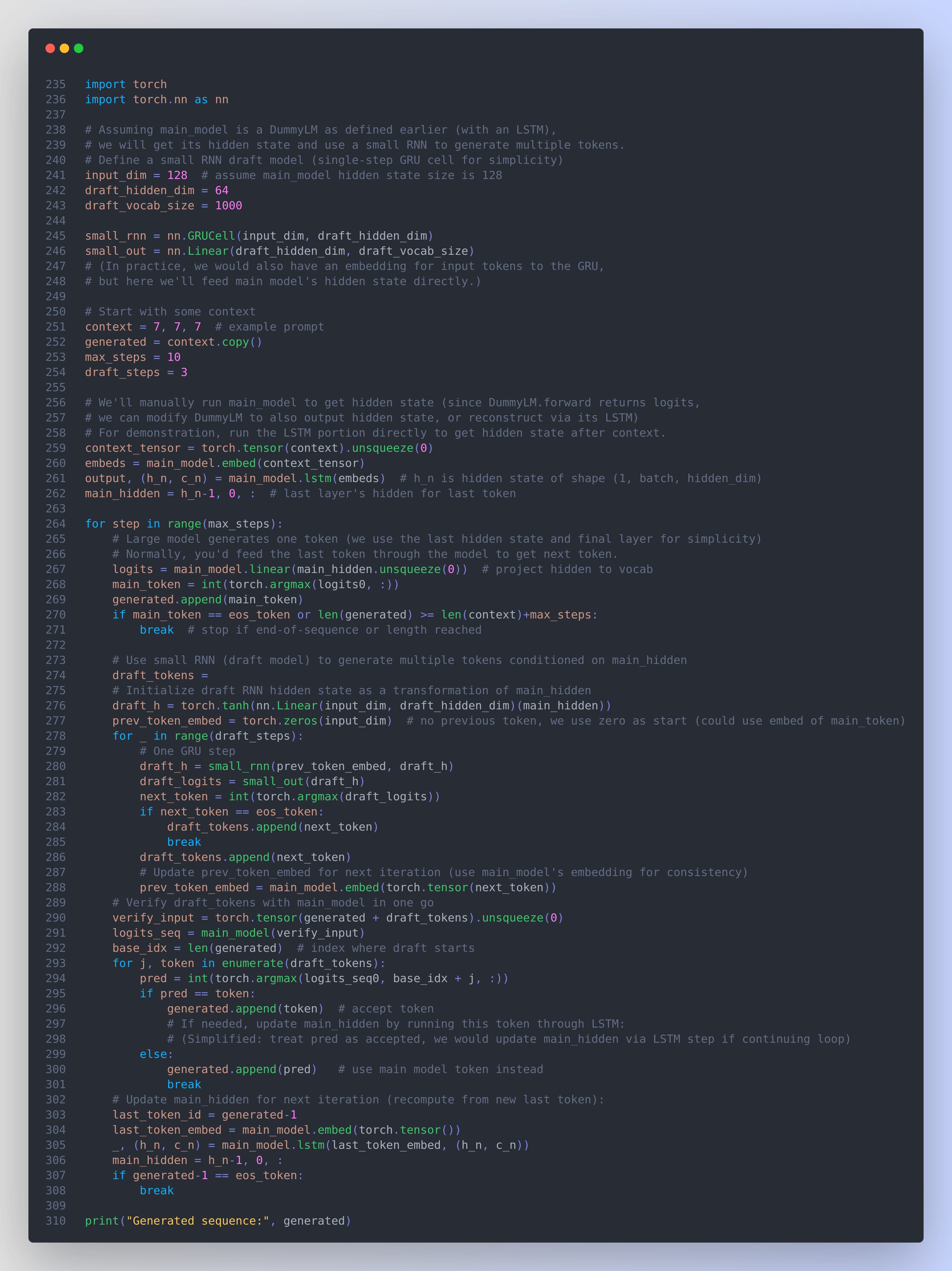
In this code, we obtain the main model’s LSTM hidden state (main_hidden) after the current context. We then generate main_token (the next token) directly from that hidden state. Next, we run a small GRU-cell-based draft model (small_rnn) for a few steps (draft_steps) to propose additional tokens. The draft model’s hidden state is initialized as a simple transformation of the main model’s hidden state, meaning it’s conditioned on the context and the just-generated main token. After generating the draft tokens, we verify them by running the main model on the extended sequence (the current output plus all draft tokens). We check each draft token against the main model’s prediction (pred), accepting those that match and breaking at the first mismatch (where we instead take the main model’s token). This approach effectively allows the small model to fast-forward the sequence by draft_steps tokens beyond the one token guaranteed by the main model. We then update the main model’s hidden state to correspond to the new context (in a real model, we would use the model’s internal caching mechanism to append the new tokens without recomputing everything from scratch).
This hybrid approach demonstrates how a smaller model (here a simple RNN) can leverage the large model’s internal state to safely accelerate generation. Many variations on this theme exist. For example, one can perform a beam search in the draft model (proposing multiple alternate continuations) and have the large model verify which beam extends the farthest without error. Alternatively, as in FIRP (Wu et al., 2024), one can predict future transformer hidden states using a lightweight model (like a linear projector) inside the large model’s layers to generate multiple tokens in a single forward pass. FIRP essentially lets the model “peek ahead” by inferring what the hidden state would be after an unseen next token, allowing it to produce that token without waiting for a new forward pass. Such methods achieved around 1.9×–3× speedups on various models. These innovations show that by using smaller or auxiliary models to anticipate the large model’s computations, one can skip redundant work and generate text significantly faster.
Where it fits in the pipeline: Fast-forwarding techniques with smaller models often require custom modifications to the model or the inference loop. In a deployment pipeline, they fit as an enhancement of the decoding step. For example, Medusa’s extra heads become part of the model architecture and are invoked inside each decoding step (the pipeline remains a single-model pipeline, but the model does more in one step). ReDrafter’s approach introduces an auxiliary model and a more complex decode function that involves both models and possibly beam search; this would be implemented as a specialized decoder module rather than a simple loop. These methods can be seen as plugin replacements for the standard decoding loop – one would integrate them into the model server such that when a generation request comes in, the server uses the advanced speculative decoder instead of naive next-token decoding. They tend to require more engineering (for example, maintaining hidden state between the large and small model, or ensuring both models’ caches and states stay in sync), as well as additional training for new components (draft model, extra heads, etc.). The payoff is fewer iterations and lower latency. These approaches particularly shine when the small model can be made extremely fast (e.g., a single-layer RNN or linear predictor) and when the large model is very expensive to run step-by-step. They represent the cutting edge of optimizing decoder-only LLM inference, pushing towards the theoretical minimum number of steps needed to generate a sequence without sacrificing output quality.
Budget Conscious Implementation Strategies
Not every deployment has abundant computational resources. Here we discuss strategies to implement speculative decoding optimizations in low-resource or budget-constrained environments:
Use quantization and efficient model formats: Reducing the memory and compute footprint of both the large and draft models is crucial on limited hardware. Quantization (e.g. 8-bit or 4-bit weights) can drastically cut memory usage. A smaller draft model can often be quantized aggressively with minimal impact on its guidance capability, since even a slightly less accurate draft still provides speedup as long as it predicts reasonably well. For example, one could load a 2-bit quantized 1B-parameter draft model alongside a 8-bit quantized 7B main model on a single GPU – the reduced precision might lower acceptance rate a bit, but if it stays high enough, the overall speed boost remains worthwhile. Additionally, one can use distilled or compressed versions of models; many draft models are themselves distilled from the target LLM, so they are already smaller and faster.
Limit draft length or strategy based on hardware: On a constrained device (like a single CPU or a mobile GPU), generating a very long draft sequence might not be beneficial because the draft model’s cost starts to loom larger. In such cases, using a small draft length (maybe 2–3 tokens at a time) or even a single-token draft can still give some speedup by parallelizing that single token’s verification with the next token’s drafting. The idea is to find a sweet spot where the draft model’s runtime is a fraction of the main model’s. If the draft model is too slow relative to the main model on your hardware, you might actually lose time drafting. So, on CPU-only scenarios, one might choose a much smaller draft model or none at all. On GPU, one could choose the draft length adaptively: e.g., if the prompt is short or the model is smaller, use a smaller draft batch to avoid overhead.
Leverage CPU/GPU concurrency: If the hardware allows, run the draft model on the CPU in parallel while the GPU is busy with the main model’s previous step. For instance, after the main model produces a token, you can have the CPU immediately start computing the next draft proposal (with a small model) while the GPU might be doing other tasks or memory transfers. By the time the GPU is ready for the next verification, the draft is ready. This kind of pipeline parallelism can hide the draft model latency. Conversely, if the GPU has spare memory but the CPU is slow, load both models on the GPU and switch between them – the overhead of context switching on GPU is low if models are small, and you avoid moving data between devices. Some serving frameworks partition the GPU for multiple models or run them in different CUDA streams to overlap their execution (the vLLM system, for example, could intermix draft model compute with main model compute in its scheduler).
If no suitable small model is available: In some cases (especially with proprietary or very new large models), you might not have a well-matched draft model readily available. Training one from scratch could be resource-prohibitive. As a budget-conscious alternative, you could use a smaller model from a previous generation or a different provider as the draft, accepting some drop in alignment. If vocabularies differ, you can sometimes map tokens or use byte-level models as a common ground. Another trick is to use partial output from the large model as a draft: for example, run the large model with a reduced number of layers to get a quick-and-dirty next token guess, then verify with the full model. This effectively uses the large model’s first few layers as a “draft model.” OpenAI’s own infrastructure reportedly does something similar (a thought: they could use a 2-layer version of GPT as a fast draft for the full GPT). While this isn’t common in literature, it’s a pragmatic hack if you cannot maintain a separate model. The TensorRT-LLM library from NVIDIA supports a variant of speculative decoding where you use the large model’s early layer outputs to predict tokens, which aligns with this idea (EAGLE - Google Sites).
Simplify and reuse components: In low-resource settings, aim to reuse the same cache and data structures for both models to save memory. For example, use a unified vocabulary and tokenizer for both models (to avoid memory overhead and conversion cost). If possible, use the same embedding layer for the draft model – e.g., initialize the draft model’s word embeddings from the large model’s (if they share vocab), then keep them fixed. This reduces memory and can improve alignment. Also consider running both models in the same process to avoid IPC overhead; lightweight draft models can be a simple function call in the code.
Profile and tune acceptance rate vs. overhead: If you only have one GPU, profile how long the draft model takes relative to the main model. If the draft model is too slow, the speculative decoding might provide little benefit or even hurt (because you’re essentially running two heavy models serially). In such cases, either downsize the draft model further (even if it becomes less accurate) or reduce the number of tokens it drafts per iteration. A slightly lower acceptance rate (meaning the main model corrects more often) can be acceptable as long as the overhead of drafting is sufficiently low. The goal is maximizing goodput – the rate of accepted tokens per unit time. A budget-limited deployment should tune parameters (draft model size, draft length, etc.) to maximize goodput on their specific hardware. Tools like the survey by Xia et al. (2024) provide guidance on how different factors (e.g., draft model quality vs speed) affect overall performance.
Use simpler speculative methods if needed: If memory or complexity is a big issue, one might opt for approximate speculative decoding that doesn’t require a full second model. For example, prompt lookup tables or n-gram caches (if the domain is predictable) can be used to guess a couple of tokens ahead. These guesses can then be verified by the main model. It’s like a poor man’s draft model using caching. While not as generally effective as a learned model, in a restricted domain it can provide a boost. Another simple method is deterministic speculation: if the model is sampling and temperature is low, often the top prediction is taken. In such cases, just take the argmax token as “draft” and have the model verify it – essentially doing speculative decoding with a trivial draft heuristic. This is almost free and can still save time if the model usually would generate that token anyway.
In summary, budget-conscious implementations should focus on smaller, maybe less accurate drafts that are extremely fast, careful device placement, and avoiding any overhead that outweighs the saved compute. Even in low-resource settings (e.g., mobile or edge devices), a modest speculative decoding setup can provide noticeable latency reductions, as evidenced by ReDrafter’s results on Apple Silicon where a memory-bound M2 chip saw 2.3× faster generation.
Startup vs Large Scale Deployment
The considerations for using speculative decoding optimizations differ between a small startup-style deployment and a large-scale production deployment:
Startup scenario (single model or small cluster, limited QPS): In a startup or development setting, you may have a single GPU (or even just CPU) serving requests, and throughput demands are low. The priority here is often latency for a single request and ease of implementation. A few guidelines in this scenario:
Choose simpler configurations: Use one small draft model for one large model, with a fixed draft length. For example, pair a 7B parameter draft with a 70B parameter model, draft maybe 2–5 tokens at a time. This straightforward approach (as we coded above) can nearly halve the response time for long outputs. There’s no need to implement complex multi-model selection or dynamic strategies until you have higher traffic.
Leverage existing libraries: Frameworks like vLLM, TensorRT-LLM, or HuggingFace’s text-generation inference server have options for speculative decoding. A startup can enable these rather than writing everything from scratch. This saves engineering effort and yields near state-of-the-art performance. For instance, vLLM’s speculative decoding can be turned on to instantly get up to ~2.8× boost in generation speed on a single GPU, as their blog reports (How Speculative Decoding Boosts vLLM Performance by up to 2.8x | vLLM Blog). Using such tools also positions you well to scale later.
Monitor and tune on real data: In a small-scale deployment, you likely have variability in request types. Keep an eye on the acceptance rate and speedup for your real traffic. If you find that for some queries the draft model is causing slowdowns (e.g., always getting rejected early), you can put in simple logic to fall back to normal decoding for those cases. For example, if a prompt is extremely domain-specific and the draft model (trained on general data) struggles, the system could detect a streak of rejections and disable speculative decoding for that request to save the wasted draft computation.
Resource trade-off: If you have only one GPU, consider running the draft model on CPU to free the GPU for the heavy model. However, if CPU is too slow, it might increase overall latency. An alternative is running both models on the GPU but alternating: for instance, load the draft model only when needed (this could still be expensive due to load time). Ideally, keep both in memory if possible to avoid loading weights each time – memory might be the limiter though. If the GPU can’t fit both models at once, a startup might opt to use a slightly smaller main model so that a draft model can be accommodated, achieving a net win in latency. For instance, using a 40B model with a 7B draft might be faster (and cheaper) than a 70B model alone, while giving similar quality output.
Don’t neglect simple batching: Even at a startup, you might have bursts of a few simultaneous requests. Batching two or three requests together for the large model can significantly improve throughput per GPU-hour. If using speculative decoding, you can batch at the verification stage easily (as shown above). The draft stage could be done separately for each (which is fine if those models are on CPU), or you could batch draft model calls too if they share a device. Implementing a small batch queue with a short delay (e.g., 5–10ms) can allow grouping requests with minimal added latency. This is essentially a mini version of what large-scale systems do, but at a scale and timeout that makes sense for a single server. It can improve utilization and reduce average latency under load.
Large-scale production (distributed servers, high QPS, strict SLAs): In a large-scale deployment, such as a cloud service serving thousands of requests per second with large LLMs, the goals are maximizing throughput, reducing cost, and ensuring latency consistency. Speculative decoding becomes one tool among many in a complex optimization pipeline:
High-throughput batching: Production systems will aggressively batch requests and even batch tokens across requests (as done in Microsoft’s and Meta’s systems, for example). In this context, speculative decoding needs to integrate with the batching mechanism. Systems like vLLM use continuous batching where incoming queries are combined on the fly. With speculative decoding, vLLM had to modify its scheduler to support multiple tokens per request in one batch slot. Production services will do similar, effectively implementing something akin to our batched code but on steroids, with dozens of requests and perhaps varying draft lengths. This requires custom CUDA kernels, efficient padding strategies, and careful memory management to avoid fragmentation when dealing with many sequences of different lengths (BASS: Batched Attention-optimized Speculative Sampling). Companies like Amazon (in BASS) and NVIDIA have invested in these optimizations. For instance, NVIDIA’s TensorRT-LLM provides an implementation of speculative decoding that works with their highly optimized transformer engine kernels, allowing nearly the theoretical max throughput on their hardware.
Distributed model deployment: Large deployments often shard very large models across GPUs (model parallelism) or use pipeline parallelism. Integrating a draft model can mean deploying an additional set of workers or processes for the draft. SPIN (2025) architecture is instructive: it introduces multiple small speculative model instances and a controller that selects which to use per request, then a pipelining so that while one batch is in the large model, another batch is being drafted on a different GPU. It essentially creates an assembly line: draft on small model GPUs, then verify on big model GPUs, with careful scheduling so each GPU is as busy as possible. In large clusters, you might dedicate some GPUs to running the draft model(s) and others to the main model, sending data between them. This adds network overhead, so it’s used when the speedups outweigh communication cost (usually within the same server or across NVLink-connected GPUs). An alternative is to co-locate a small and large model on each GPU if memory permits and run them sequentially on device. The best choice depends on model sizes and GPU memory. If the main model is extremely large (filling most of the GPU), using separate GPUs for the draft is preferable.
Caching and KV management: Large models benefit greatly from caching past key/value tensors for the self-attention layers, to avoid recomputing those for each new token. Speculative decoding complicates this slightly: when multiple tokens are accepted in one go, you need to update the cache with all of them at once. Frameworks handle this by either unrolling the verification internally or by computing the new keys/values for all accepted tokens in one batch. For production, it’s crucial that the caching mechanism supports adding a variable number of tokens. vLLM’s memory manager was explicitly extended to handle caching for speculative decoding – it needs to store KV caches for both the draft and main models and be able to append to the main model’s cache multiple tokens at a time. Efficient cache management avoids recomputation of context and keeps latency low even as sequence lengths grow.
Robustness and fallback: At scale, you care about tail latency (the slowest requests). If the draft model occasionally misfires (e.g., predicts a long sequence that mostly gets rejected, causing extra work), that could hurt the 99th percentile latency. Production systems might implement a timeout or fallback: if the speculative decoding isn’t making progress fast enough, they can revert to normal decoding for the remainder of that request. Another strategy is to use a smaller draft length when the system is under heavy load to ensure no single request hogs the GPU with a long speculative verification. Essentially, large-scale systems use empirical data to finely tune parameters (draft lengths, model sizes, etc.) to balance speedup vs. risk. They might also maintain different draft models for different scenarios (as SPIN does) and choose them based on the prompt or known difficulty of the task.
Cost trade-offs: Large deployments are usually cost-sensitive. Running an extra model has a cost in GPU hours. The decision to use speculative decoding at scale comes down to throughput per dollar. If a draft model uses 10% extra GPU memory and 20% extra compute but doubles the throughput, it’s a net win. But if the draft model has to be too big (say 50% the size of the main model) to get a good acceptance rate, some platforms might instead run two instances of the main model in parallel and achieve similar throughput. That’s why research has focused on making draft models as small as possible while still effective. A large service might experiment with several configurations (e.g., a 2B draft vs a 6B draft paired with a 70B model) to see which gives the best throughput/cost. They’ll also consider maintenance cost: an extra model means extra complexity in updates and monitoring. The survey by Xia et al. (2024) notes that draft model latency and alignment are the key factors, not just perplexity or quality of the draft model itself. So a production team will choose a draft model that perhaps is less powerful in language ability if it runs significantly faster or uses less memory, because that yields better overall service efficiency.
In large-scale deployments, speculative decoding is often combined with other optimizations: e.g., model distillation (serving a slightly distilled faster model with minimal quality drop), request batching, and hardware-specific accelerations. It’s one piece of a larger puzzle to serve LLMs at scale. The consensus in recent literature (2024–2025) is that speculative decoding significantly boosts throughput and is becoming a standard part of LLM serving infrastructure. As long as the engineering challenges are addressed (which recent research and toolkits are actively doing), both startups and large enterprises can benefit from these strategies – with startups focusing on quick wins like a single draft model, and large-scale deployments leveraging the full spectrum (batched, heterogeneous drafts, pipelining) to squeeze maximum performance out of their hardware.