
The mean, the median, and mode of a Random Variable

The mean is called a measure of central tendency because it tells us something about the center of a distribution, specifically its center of mass. Other measures of central tendency that are commonly used in statistics are the median and the mode, which we now define.
These are three statistical quantities that we are frequently interested in: mean, mode, and median. We all know how to compute these from a dataset. For example, to compute the median of a dataset, we sort the data and pick the number that sits in the 50th percentile. However, the median computed in this way is the empirical median, i.e., it is a value computed from a particular dataset. If the data is generated from a random variable (with a given PDF), how do we compute the mean, median, and mode?
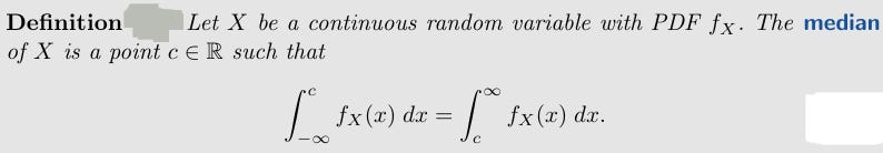
Here’s the definition of Median and CDF is Cumulative Distribution Function and PMF is Probability Mass Function.
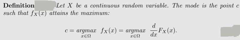
And for Mode
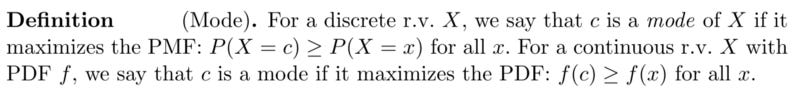
Intuitively, the median is a value c such that half the mass of the distribution falls on either side of c (or as close to half as possible, for discrete r.v.s), and the mode is a value that has the greatest mass or density out of all values in the support of X. If the CDF F is a continuous, strictly increasing function, then
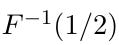
is the median (and is unique).
Note that the mode of a random variable is not unique, e.g., a mixture of two identical Gaussians with different means has two modes.
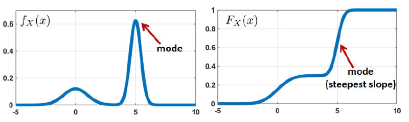
In above figure Left — The mode appears at the peak of the PDF.
And in the Right figure, the mode appears at the steepest slope of the CDF.
Note that a distribution can have multiple medians and multiple modes. Medians have to occur side by side; modes can occur all over the distribution.
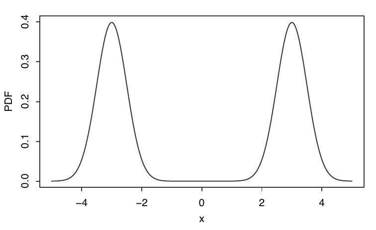
In below figure, I show a distribution supported on [−5, −1] ∪ [1, 5] that has two modes and infinitely many medians. The PDF is 0 between −1 and 1, so all values between −1 and 1 are medians of the distribution because half of the mass falls on either side. The two modes are at −3 and 3.
When is the mean the best measure of central tendency?
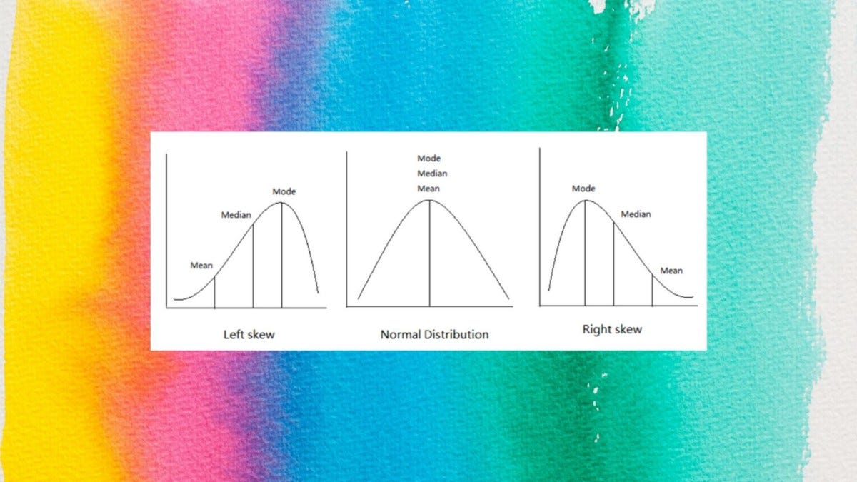
The mean is usually the best measure of central tendency to use when your data distribution is continuous and symmetrical, such as when your data is normally distributed.
When is the mode the best measure of central tendency?
The mode is the least used of the measures of central tendency and can only be used when dealing with nominal data.
Nominal variables are variables that have two or more categories, but which do not have an intrinsic order. For example, a real estate agent could classify their types of property into distinct categories such as houses, condos, co-ops or bungalows. So “type of property” is a nominal variable with 4 categories called houses, condos, co-ops and bungalows.
When is the median the best measure of central tendency?
The median is usually preferred to other measures of central tendency when your data set is skewed (i.e., forms a skewed distribution) or you are dealing with ordinal data. However, the mode can also be appropriate in these situations, but is not as commonly used as the median.
Lets do a quick example on Mean, median, and mode for salaries. A certain company has 100 employees. Let s1, s2, . . . , s100 be their salaries, sorted in increasing order (we can still do this even if some salaries appear more than once). Let X be the salary of a randomly selected employee (chosen uniformly). The mean, median, and mode for the data set s1 , s2 , . . . , s100 are defined to be the corresponding quantities for X.
What is a typical salary? What is the most useful one-number summary of the salary data? The answer, as is often the case, is it depends on the goal. Different summaries reveal different characteristics of the data, so it may be hard to choose just one number — and it is often unnecessary to do so, since usually we can provide several summaries (and plot the data too). Here we briefly compare the mean, median, and mode, though often it makes sense to report all three (and other summaries too).
If the salaries are all different, the mode doesn’t give a useful one-number summary since there are 100 modes. If there are only a few possible salaries in the company, the mode becomes more useful. But even then it could happen that, for example, 34 people receive salary a, 33 receive salary b, and 33 receive salary c. Then a is the unique mode, but if we only report a we are ignoring b and c, which just barely missed being modes and which together account for almost 2/3 of the data.
Next, let’s consider the median. There are two numbers “in the middle”, s50 and s51 . In fact, any number m with s50 ≤ m ≤ s51 is a median, since there is at least a 50% chance that the random employee’s salary is in {s1 , . . . , s50 } (in which case it is at most m) and at least a 50% chance that it is in {s51 , . . . , s100} (in which case it is at least m). The usual convention is to choose m = (s50 + s51 )/2, the mean of the two numbers in the middle. If the number of employees had been odd, this issue would not have come up; in that case, there is a unique median, the number in the middle when all the salaries are listed in increasing order.
Compared with the mean, the median is much less sensitive to extreme values. For example, if the CEO’s salary is changed from being slightly more than anyone else’s to vastly more than anyone else’s, that could have a large impact on the mean but it has no impact on the median. This robustness is a reason that the median could be a more sensible summary than the mean of what the typical salary is. On the other hand, suppose that we want to know the total cost the company is paying for its employees’ salaries. If we only know a mode or a median, we can’t extract this information, but if we know the mean we can just multiply it by 100.