
The relationship between Curse of Dimensionality and Degrees of Freedom

Degrees of Freedom
Degrees of Freedom (DoF) refers to the number of independent parameters or variables in a model or system. It represents the flexibility of the model to adapt to the data. In the context of statistical modeling, DoF is often used to assess the complexity of a model, with more complex models having higher DoF.
The dimension of a mathematical object is the number of independent variables needed to fully describe it. A point has 0 dimensions. A line has 1 dimension, a square has 2 dimensions and a cube has 3 dimensions. On a line we need one variable, let’s say the distance from a starting point in order to pinpoint our position. On a square we need at least 2 pieces of information (x and y). In a cube, we need 3 coordinates (x,y,z)
Now, I will try to give a intuitive interpretation of degrees of freedom in the context of Data Science.
The number of degrees of freedom you have describes your uncertainty.
If I am given two people's names (Mr A and Mr B) and asked their ages, I know neither: So in this case, I have 2 degrees of freedom, one for each age. If I am then told that Mr X's age is 20, I still don't know Mr Y's age: 1 degree of freedom removed, 1 left. I am then told that their mean age is 30. This constraint removes the last degree of freedom and I know that Mr Y must be 40 years old.
Each time you find out (or set) something about the system you are working with, such as a value or a parameter (such as the mean illustrated here), this decreases the number of degrees of freedom by 1.
Degrees of freedom is a fundamental concept in statistics and data science that represents the number of independent pieces of information available in a sample for estimating certain parameters or making statistical inferences. In other words, DF can be seen as the number of "free" choices that can be made in a calculation without violating any constraints or conditions.
Understanding DoF with Vector
If I have a vector of length 10 that can take any values, then I need all the 10 coordinates to know about the vector is, and so in that means, there are 10 degrees of freedom.
Now, If I am told that the sum of the elements of the vector is zero, then any 9 of the coordinates determine the tenth, and so now the number degrees of freedom becomes 9
The key idea is that the degrees of freedom is the minimum number of values that you need to specify a quantity. If you're comfortable with geometry in the abstract, you can think of the degrees of freedom as the dimension of the space that the numbers "live in".
Let's consider some examples to illustrate the concept of degrees of freedom in different contexts:
Example: Room Temperature
Imagine you have a room with four heaters, and you can control the temperature of each heater individually. You are asked to maintain the average temperature in the room at 80 degrees Fahrenheit. In this case, you have the freedom to choose the temperature of the first three heaters independently. However, the temperature of the fourth heater is constrained by the condition of maintaining an average room temperature of 80 degrees Fahrenheit.
Suppose you set the temperatures of the first three heaters as follows:
Heater 1: 85°F Heater 2: 70°F Heater 3: 90°F
The average temperature of these three heaters is (85 + 70 + 90) / 3 = 81.67°F. To maintain an average room temperature of 80°F, the temperature of the fourth heater must be set to:
Heater 4: 80 - (81.67 - 80) = 78.33°F
In this example, you have 3 degrees of freedom, as there were 3 independent choices (the temperatures of the first three heaters), while the fourth heater's temperature is constrained by the condition of maintaining an average room temperature of 80°F.
Linear Regression:
In the context of linear regression, degrees of freedom help us understand how much information is available for estimating the model parameters (i.e., the coefficients and the intercept) and quantifying the uncertainty around these estimates.
For a simple linear regression with one independent variable (x) and one dependent variable (y), we estimate two parameters: the slope (β) and the intercept (α). In this case, the degrees of freedom are calculated as:
DF = n - p
where 'n' is the number of observations in the dataset and 'p' is the number of estimated parameters (including the intercept).
Example: If we have a dataset with 20 observations and we're fitting a simple linear regression model (with one independent variable and an intercept), the degrees of freedom would be:
DF = 20 - (1 + 1) = 18
The 18 degrees of freedom represent the amount of "free" information available for estimating the model parameters and characterizing the uncertainty around these estimates.
T-Test:
When comparing the means of two samples using a t-test, degrees of freedom play a crucial role in determining the appropriate t-distribution to use for hypothesis testing.
For an independent two-sample t-test, the degrees of freedom are calculated as:
DF = n1 + n2 - 2
where 'n1' and 'n2' are the sample sizes of the two groups being compared.
Example: Suppose we want to compare the means of two groups, Group A with 15 observations and Group B with 20 observations. In this case, the degrees of freedom for the t-test would be:
DF = 15 + 20 - 2 = 33
The 33 degrees of freedom inform the t-distribution that we will use to conduct the t-test and draw conclusions about the statistical significance of the difference in means between the two groups.
In summary, degrees of freedom is a fundamental concept in data science that helps us understand the amount of independent information available for estimating parameters or making statistical inferences. It is essential for characterizing the uncertainty around these estimates and informing the appropriate statistical distributions used in hypothesis testing.
Statisticians/Data scientists often say "Don't add more variables, you won't have enough degrees of freedom."
Let's understand this statement using multi linear regression as an example. In multi linear regression, adding more independent variables reduces the degrees of freedom.
The more variables you have, the higher the amount of variance you can explain. Even if each variable doesn't explain much, adding a large number of variables can result in very high values of R2. This is why some packages provide "Adjusted R2," which allows you to compare regressions with different numbers of variables.
The same holds true for polynomial regression. If you have N data points, then you can fit the points exactly with a polynomial of degree N-1.
The degrees of freedom in a multiple regression equals N-k-1, where k is the number of variables or the numbers of parameters you're estimating.
The additional -1 in the formula is for the intercept - it's an additional predictor. So, the residual vector will exist in an n−k-1 dimensional linear space.
However, in simple linear regression you estimate both a y-intercept and a slope, so k=2. Even though we generally don't worry about testing the intercept, it still uses up a degree of freedom, the slope would be very different and have a very different interpretation if we did not estimate an intercept along with the slope.
The more variables you add, the more you erode your ability to test the model (e.g. your statistical power goes down).
As we add more variables, the DF decreases, leading to a higher variance of the parameter estimates, and consequently, wider confidence intervals for those estimates. This may result in less precise conclusions about the relationships between the independent and dependent variables.
This phenomenon is closely related to the "curse of dimensionality," where adding more variables equates to adding more dimensions.
You might wonder - why is it a curse? The problem is that if we add more parameter to a multiple Linear Regression, but out input data remains the same - it will make it sparse at higher dimensions.
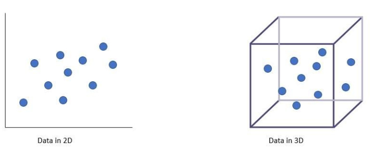
The image below illustrates how the same number of data points looks dense in 2D but sparse in 3D. Imagine the sparsity in higher dimensions!
We need more data to fill up the space, but often, the data at hand is limited.
Adding more variables leads to:
Loss of degrees of freedom.
Highly inflated R squared value.
Curse of Dimensionality
As the number of dimensions (features) in a dataset increases, the complexity of the problem grows exponentially, making it more difficult to gain insights or build accurate models.
Some issues related to the Curse of Dimensionality include:
Sparse sampling: As the number of dimensions increases, the amount of data needed to cover the space grows exponentially. This results in sparse sampling, where data points become increasingly distant from each other, making it challenging to identify meaningful patterns or relationships.
Increased computational complexity: High-dimensional data requires more computational resources and time to process, which can be prohibitive, particularly for algorithms with a high time complexity.
Overfitting: In high-dimensional spaces, models can become overly complex, capturing noise rather than the underlying data structure, leading to poor generalization to new data. Overfitting can be explained through the bias-variance trade-off. As we add more variables to a model, we reduce its bias (the systematic error in the model's predictions) but increase its variance (the sensitivity of the model to small fluctuations in the data).
Model Interpretability: Adding more variables to a model can decrease its interpretability, as it becomes more challenging to disentangle the effects of individual variables on the response.
Relationship between Curse of Dimensionality and Degrees of Freedom
The relationship between the Curse of Dimensionality and Degrees of Freedom can be understood in the context of model complexity and overfitting.
Model complexity: As the number of dimensions (features) in a dataset increases, the Degrees of Freedom in a model also increases. This is because the model has more parameters or variables to adjust to fit the data. This added flexibility can lead to an increased risk of overfitting, as the model may adapt too well to the training data, capturing noise rather than the underlying structure.
Overfitting: Overfitting is a direct consequence of the Curse of Dimensionality and high Degrees of Freedom. In high-dimensional spaces, models with high DoF can fit the training data too closely, leading to poor generalization to new, unseen data. Regularization techniques, such as Lasso or Ridge Regression, can be applied to reduce the model's complexity and mitigate overfitting.