Read time: 16 min
📚 Browse past editions here.
( I publish this newletter daily. Noise-free, actionable, applied-AI developments only).
⚡Top Papers of last week (28-Sept-2025 ):
🗞️ ARE: scaling up agent environments and evaluations
🗞️ Hierarchical Retrieval: The Geometry and a Pretrain-Finetune Recipe
🗞️ Single-stream Policy Optimization
🗞️ LIMI: Less is More for Agency
🗞️ MetaEmbed: Scaling Multimodal Retrieval at Test-Time with Flexible Late Interaction
🗞️ Video models are zero-shot learners and reasoners
🗞️ Federation of Agents: A Semantics-Aware Communication Fabric for Large-Scale Agentic AI
🗞️ ARE: scaling up agent environments and evaluations
🧠 Great research from Meta Superintelligence Labs. Proposes Meta Agents Research Environments (ARE) for scaling up agent environments and evaluations.
ARE lets researchers build realistic agent environments, run agents asynchronously, and verify them cleanly. On top of it they release Gaia2, a 1,120 scenario benchmark that stresses search, execution, ambiguity, time pressure, collaboration, and noise, and the results show sharp tradeoffs between raw reasoning and speed or cost.
⚙️ The Core Concepts
ARE (Agent Runtime Environment) treats the world as a clocked simulation where everything is an event, the agent runs separately, and interactions flow through tools and notifications. Apps are the tools, environments bundle the apps plus rules, and scenarios package starting state, scheduled events, and a verifier.
Traditional old benchmarks froze the world while a model was “thinking.” That made results look clean but ignored the real costs of inference time.
In ARE, the world keeps ticking asynchronously. Time passes even while the model is generating, apps can trigger notifications, and other actors may act. So if a model is slow, it directly shows up as missed deadlines in the benchmark.
That is exactly why GPT-5 (high) got 79.6 on Search but 0 on Time in default mode. The reasoning quality was excellent, but ARE exposed its inference slowness as a concrete failure mode.
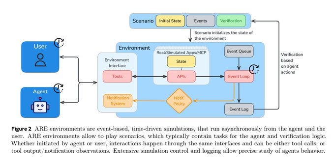
When ARE switched to instant mode, stripping out the latency, the model suddenly performed well — proving the bottleneck wasn’t reasoning but raw response time. This figure shows that ARE (Agent Runtime Environment) runs as an event-based simulation where both agent and user interact through the same interface.
The environment manages tools, APIs, state, and a notification system, with everything logged in an event queue. Scenarios define the starting state, scheduled events, and verification rules, while the event loop keeps moving regardless of agent speed. Because of this, if the agent is slow, the world continues and actions can be judged late or wrong, which directly exposes latency problems like those seen with GPT-5 (high).
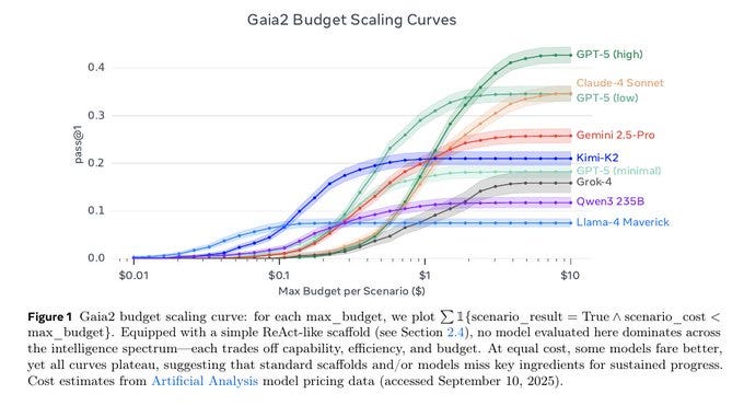
This graph is showing how different models perform in Gaia2 when you also take into account the money spent per task.
The y-axis is pass@1, which means the fraction of scenarios solved on the first attempt. The x-axis is max budget per scenario, basically the upper limit of how much you are willing to spend on model calls to solve one benchmark task.
As the budget rises, models get more space to “think” and call tools, so pass@1 improves. But after a certain point, every curve plateaus. That means throwing more money at the same scaffold does not buy more performance. The model has hit its natural limit under that setup. key takeaway is that no single model dominates across both cost and capability.
🗞️ Hierarchical Retrieval: The Geometry and a Pretrain-Finetune Recipe
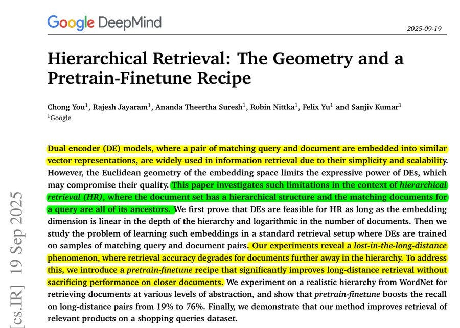
Brilliant GoogleDeepMind paper, a major advancement in embedding-based search. Most regular search systems return only exact or near matches, they miss those farther-up categories that still matter, the bigger parent categories your query belongs to.
And this paper’s simple 2-step training pulls those in reliably, lifting far-away match accuracy from 19% to 76%. Meaning, the Long-distance recall jumps from 19% to 76% on WordNet with low-dimensional embeddings.
Long-distance recall is the % of the far-away relevant items that your search actually returns. “Far-away” means items several steps up the category tree from your query, like “Footwear” for “Kid’s sandals”.
You compute it by looking only at those distant ancestors, counting how many should be returned, counting how many you actually returned, then doing hits divided by should-have. If there are 10 such ancestors and your system returns 7, long-distance recall is 70%.
⚙️ The Core Concepts
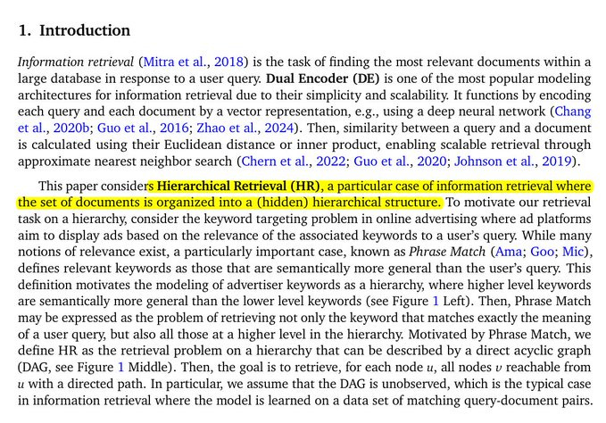
Hierarchical retrieval expects a query to bring back its own node and all more general ancestors, which is asymmetric, so the same concept must embed differently on the query side and the document side. Euclidean geometry creates tension across queries, yet an asymmetric dual-encoder can resolve it with careful scoring. The running example is “Kid’s sandals,” where “Sandals” is relevant to that query, but the reverse is not, which motivates asymmetric scoring.
🧠 The idea of this paper.
Dual encoders can solve hierarchical retrieval when query and document embeddings are asymmetric and the needed dimension grows gently with hierarchy depth and log of catalog size. A simple schedule, pretrain on regular pairs then finetune on long-distance pairs, fixes misses on far ancestors without hurting close matches.
🧩 Quick outline
The task is to retrieve the exact node plus all more general ancestors, so relevance is one-way. They formalize the setup, train with a softmax loss over in-batch negatives, and score by recall.
They prove feasible Euclidean embeddings exist with a dimension that scales with depth and log of size. Synthetic trees show learned encoders work at much smaller dimensions than the constructive bound.
Tiny dimensions fail mainly on far ancestors, the “lost-in-the-long-distance” effect. Up-weighting far pairs hurts near pairs, so rebalancing alone fails.
Pretrain then finetune only on far pairs lifts all distance slices with early stopping to protect near pairs. On WordNet and Amazon ESCI, the recipe gives clear recall gains across slices.
📦 Problem setup and training loss
They define a directed acyclic graph over documents, map each query to its exact document, mark every reachable ancestor as relevant, then train dual encoders with a softmax cross-entropy using temperature 20. This pushes a query to score higher with any ancestor than with unrelated items while keeping fast nearest neighbor search.
📐 Geometry result, how much dimension is enough
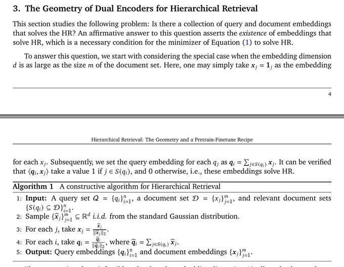
They construct embeddings by summing random unit document vectors for each query’s ancestor set and prove a single threshold separates matches from non-matches with high probability. The needed dimension grows roughly with the maximum ancestor count per query and with log of total documents, so linear in depth, logarithmic in catalog size, not in the number of queries. For a perfect tree, this turns into about depth squared times log of branching, which is still compact.
🔬 Synthetic trees, what dimension actually works
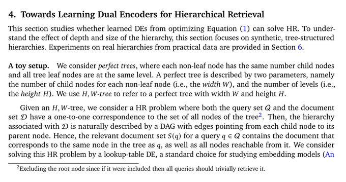
They build perfect trees with width W and height H, train lookup-table encoders with the same softmax loss, and find the smallest dimension that hits >95% recall. Learned encoders meet the target at dimensions below the constructive bound, and the fitted trend matches the theory that scales with H and log W.
📉 The “lost-in-the-long-distance” effect
With tiny dimension, models nail exact or near-parent matches yet miss distant ancestors and recall decays with query-document distance. Rebalancing by over-sampling far pairs lifts far-slice recall but torpedoes near-slice recall, showing a hard trade-off when training everything at once.
🧪 Pretrain then finetune, why this fixes it
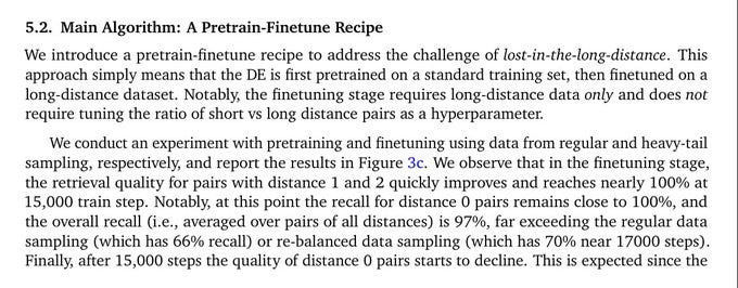
First pretrain on regular pairs to lock local neighborhoods, then finetune only on far pairs with a 1,000× lower learning rate and a higher temperature of 500, which quickly boosts far-slice recall while keeping near-slice recall intact. Early stopping prevents late drift, and the finetune does not need exact graph distances, any practical proxy that separates near from far suffices.
📚 WordNet results, long-distance retrieval finally shows up
On noun synsets, pretrain then finetune lifts every distance slice, reaching 92.3% overall recall at dimension 64 with the worst slice still at 75.7%. At dimension 16, overall recall rises from 43.0% to 60.1%, and the standout long-distance slice shows 19% → 76%.
HyperLex correlation improves to 0.415 from 0.350, indicating better graded hypernym understanding after finetune. Hyperbolic embeddings beat plain Euclidean training at the same size, yet still trail the pretrain-finetune Euclidean setup for comparable settings.
🧰 How to reproduce the recipe sensibly
Start with regular sampling, train until near-slice recall stabilizes, and save a strong checkpoint. Switch to a far-only finetune set using a simple proxy for distance, cut the learning rate by 1000×, raise the temperature to around 500, monitor slices, and stop early when all distances are high.
This figure explains hierarchical retrieval, where a query should return its ancestors in a product or concept tree. It uses “Kid’s sandals” to show asymmetric relevance, since “Sandals”, “Kid’s shoes”, and “Footwear” are correct matches upward but the reverse is not.
The graph sketch just generalizes that idea as a directed acyclic graph so ancestors are the nodes you can reach by following arrows upward. The line chart shows the core failure of standard dual encoders, recall crashes as the ancestor is farther in the hierarchy, the lost-in-the-long-distance effect.
The dashed line shows the fix, a pretrain then finetune schedule that keeps recall high even for far ancestors. The takeaway: train normally for the local structure, then finetune on far pairs to recover the long-distance matches without breaking the near ones.
Why hierarchical retrieval is tricky in the first place?
The usual way dual encoders work is by putting queries and documents into a space where closer distance means more relevance. That works fine when relevance is symmetric, like “apple” and “fruit” being related both ways.
But in hierarchies, relevance is one-directional. If the query is “Kid’s sandals”, then “Sandals” or “Footwear” should be considered relevant because they are ancestors. But if the query is “Sandals”, “Kid’s sandals” should not be returned, since it’s too specific.
This asymmetry makes the job harder. That’s why the paper says you need asymmetric embeddings, where the same concept is treated differently depending on whether it is on the query side or the document side. That’s the foundation of their whole approach.
🗞️ Single-stream Policy Optimization
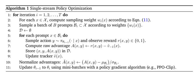
An approach that fixes GRPO’s wasted compute from degenerate groups and its constant group synchronization stalls, making training both faster and more stable.
🧠 The idea
SPO trains with 1 response per prompt, keeps a persistent baseline per prompt, and normalizes advantages across the batch, which stabilizes learning and cuts waste. This removes degenerate groups that give 0 signal and avoids group synchronization stalls in distributed runs.
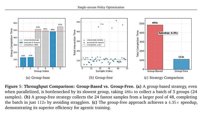
On math reasoning with Qwen3-8B, SPO improves accuracy and learns more smoothly than GRPO. Sensational fact: 4.35× throughput speedup in an agentic simulation and +3.4 pp maj@32 over GRPO.
🧩 The problem with group-based training
Group-based methods sample many responses per prompt to compute a relative baseline, but when every response in a group is all correct or all wrong the advantages become 0 and the step gives no gradient. Heuristics like dynamic sampling try to force a non-zero advantage, but they add complexity and keep a synchronization barrier that slows large-scale training.
How GRPO and SPO (Single-stream Policy Optimization) process a prompt?
In GRPO, each prompt generates multiple responses. Those responses each get rewards, and then the rewards are normalized within the group to calculate the advantage.
The problem is that if all responses are equally good or bad, the group normalization wipes out the signal, leaving no useful gradient. In SPO, a prompt produces only one response. The reward from that response is compared against a persistent value estimate for that prompt.
That difference becomes the advantage. This way, every response contributes directly to learning, and the persistent baseline keeps the updates stable instead of relying on a group comparison.
So the figure highlights why SPO is simpler and more efficient. GRPO wastes samples when groups collapse, while SPO ensures each sample matters and avoids the synchronization barrier of waiting for entire groups to finish.
🧠 What SPO changes at a high level
SPO returns to single-sample policy gradient, it uses a persistent value estimate for each prompt as the baseline instead of an on-the-fly group mean. It normalizes advantages across the whole batch, so samples of mixed difficulty share a stable scale. The persistent baseline also acts like a live curriculum signal, so sampling can focus compute where learning potential is highest.
🧪 The KL-adaptive value tracker
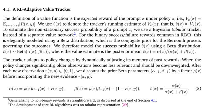
For each prompt, SPO keeps a Beta-distribution tracker of success probability and updates it like an adaptive moving average that trusts new outcomes more when the policy has changed a lot. Policy change is measured by KL divergence between the current policy and the last policy that acted on that prompt, which sets how fast old evidence is forgotten. Initialization uses a small batch of outcomes plus an effective sample size tied to the minimum forgetting rate, which prevents wild swings at the start.
⚙️ Advantage calculation and the policy loss
The advantage per sample is reward minus the tracker’s previous estimate for that prompt, which keeps the baseline independent from the action taken now. Advantages are centered and scaled across the full batch, then applied token-wise with PPO-Clip, so training stays stable without learning a separate critic of the same size as the policy. Turning off the baseline still optimizes but raises variance, which is exactly what the baseline is meant to reduce.
🎯 Prioritized prompt sampling
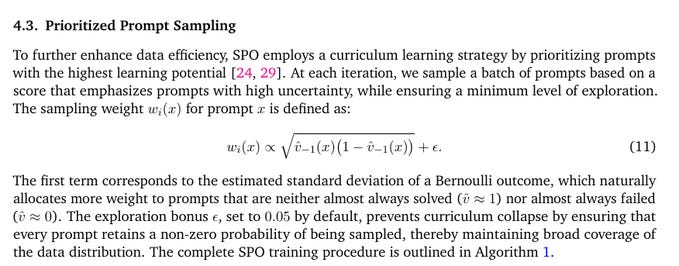
SPO samples prompts more often when the tracker is uncertain, roughly around a mid success rate, and it keeps a small exploration floor so no prompt is starved. This concentrates compute on cases that can actually change the model rather than on prompts that are already solved or currently hopeless.
🚦 Throughput in agentic settings
A group-based batch must wait for the slowest group to finish, which in the simulation means 486s to gather 24 samples, while the group-free SPO strategy collects the first 24 of 48 parallel samples in 112s, a 4.35× speedup. This asynchrony avoids stragglers and lets fast trajectories contribute immediately, which is exactly what long-horizon tool use needs.
🗞️ LIMI: Less is More for Agency
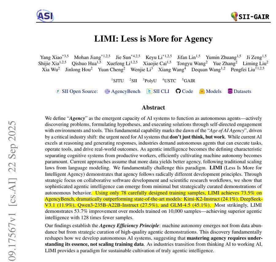
BIG claim. Giving an LLM just 78 carefully chosen, full workflow examples makes it perform better at real agent tasks than training it with 10,000 synthetic samples.
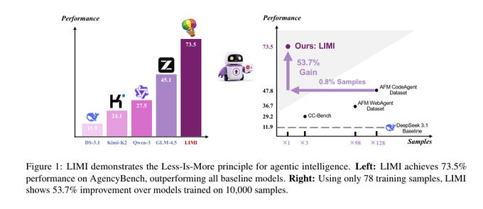
“Dramatically outperforms SOTA models: Kimi-K2-Instruct, DeepSeek-V3.1, Qwen3-235B-A22B-Instruct and GLM-4.5. “ on AgencyBench (LIMI at 73.5%)
The big deal is that quality and completeness of examples matter way more than raw data scale when teaching models how to act like agents instead of just talk. They name the Agency Efficiency Principle, which says useful autonomy comes from a few high quality demonstrations of full workflows, not from raw scale.
The core message is strategic curation over scale for agents that plan, use tools, and finish work. In summary how LIMI (Less Is More for Intelligent Agency) can score so high with just 78 examples.
1. Each example is very dense
Instead of short one-line prompts, each example is a full workflow. It contains planning steps, tool calls, human feedback, corrections, and the final solution. That means 1 example teaches the model dozens of small but connected behaviors.
2. The tasks are carefully chosen
They didn’t just collect random problems. They picked tasks from real coding and research workflows that force the model to show agency: breaking down problems, tracking state, and fixing mistakes. These skills generalize to many other tasks.
3. Complete trajectories, not fragments
The dataset logs the entire process from the first thought to the final answer. This is like showing the model not only the answer key but the full worked-out solution, so it can copy the reasoning pattern, not just the result.
4. Less noise, more signal
Large datasets often have lots of filler or synthetic tasks that don’t push real agent skills. LIMI avoids that by strict quality control, so almost every token in the dataset contributes to useful learning.
5. Scale of information per token
Because each trajectory is huge (tens of thousands of tokens), the model effectively sees way more “learning signal” than the raw count of 78 samples suggests. The richness of one trajectory can outweigh hundreds of shallow synthetic prompts.
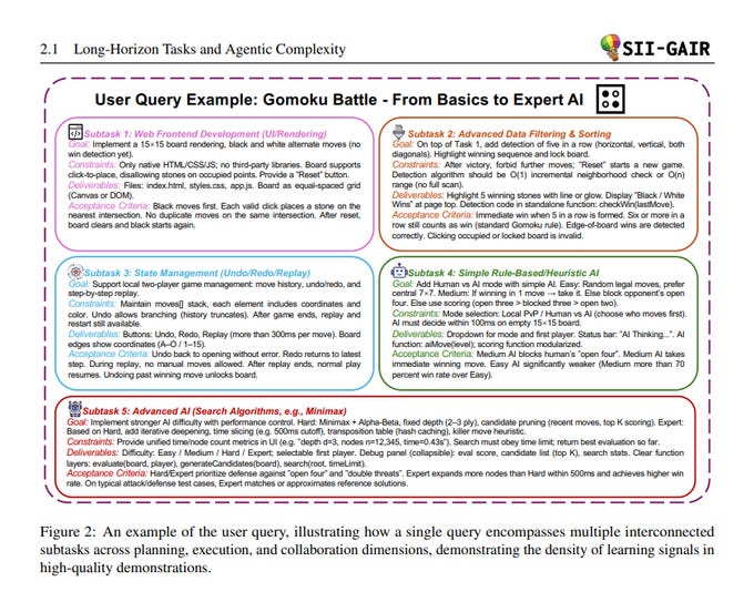
An example of the user query. Shows how a single query encompasses multiple interconnected subtasks across planning, execution, and collaboration dimensions, demonstrating the density of learning signals in high-quality demonstrations.
LIMI (Less Is More for Intelligent Agency) hits 73.5% on AgencyBench, which is way higher than other strong models like GLM-4.5 (45.1%) or Qwen-3 (27.5%). On the right, it shows the efficiency side. LIMI uses only 78 samples, which is just 0.8% of what other datasets use, yet it delivers a 53.7% improvement compared to models trained on 10,000 samples.
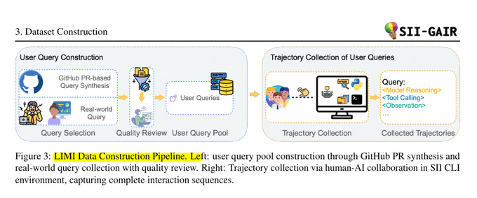
How the training data for LIMI was built?
On the left side, they show how user queries were created. Some queries come directly from real-world developer and researcher needs, while others are generated from GitHub pull requests. Every query then goes through a quality review before being added to the user query pool. This ensures that the model only trains on meaningful and realistic tasks.
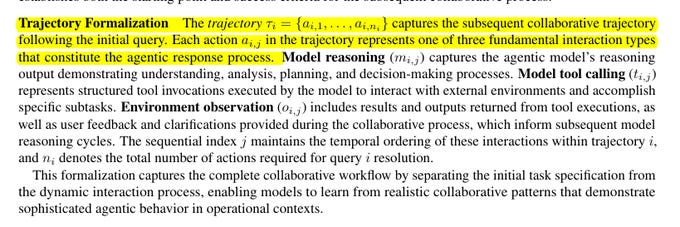
On the right side, they show how these queries are paired with complete trajectories. A trajectory is a full interaction log that captures the model’s reasoning, tool use, and observations step by step until the task is done. These are collected in the SII command line interface, with humans collaborating to guide the process and make sure full sequences are recorded. The main idea here is that the dataset does not just have short prompts, but instead contains rich, multi-step records of how problems are solved, which is exactly what helps the model learn agency.
🧩 The task settings that exercise agency
Two domains cover most knowledge work, vibe coding for collaborative software development and research workflows for literature, data, and experiments. Tasks are long horizon with many rounds, which forces decomposition, tool use, state tracking, and back-and-forth with a human partner. A single query can pack several connected subtasks, so 1 sample carries dense learning signals across planning and execution.
🗂️ How the 78 training queries were built
Most queries come from real developer and researcher needs, then a GitHub pull request pipeline adds coverage while keeping authentic context. High quality repositories are sampled, pull requests are filtered for substance, experts review semantic fidelity, and 18 pull-request items are picked to match the 2 core domains. The dataset stays tiny but rich, which proves the point that quality beats volume for teaching agent behavior.
🧭 What a “trajectory” captures
Each query is paired with a full interaction trace that interleaves model reasoning, tool calls, and environment feedback, step by step until success. Traces are gathered in the SII command line interface, with humans collaborating to steer realistic workflows and to log complete runs including recovery from mistakes. The traces are long, average 42.4K tokens and up to 152K, which exposes the model to real multi-turn execution patterns.
🧪 Benchmarks and what is measured
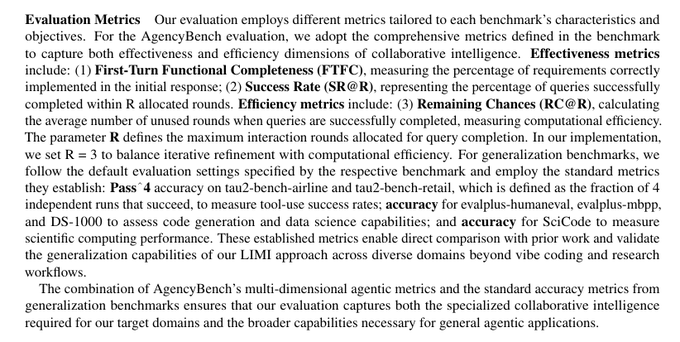
AgencyBench checks first-turn functional completeness, overall success within 3 rounds, and how many rounds remain unused when finishing early. Generalization adds tool-use tests, coding suites, data-science tasks, and scientific computing, so gains are not tied to 1 niche. Training and evaluation settings are held constant, so differences reflect data quality rather than setup tricks.
🪙 Why less data wins here
Against a 10,000 sample code-agent dataset, the 78 sample LIMI run is 53.7% higher on AgencyBench with 128x less data. The same trend holds on generalization suites, beating larger synthetic corpora while using 30% to 1% of their size. The practical rule is simple, pick tasks that teach real agent behaviors and keep the logs complete, then the model copies those patterns efficiently.
🛠️ How much the tools matter
Without any command line tools, LIMI still edges the base GLM-4.5 on the mixed benchmark average, which shows the core skill gains live inside the model. With the SII command line interface enabled, performance rises by 7.2 points because the model can express its planning and tool coordination skills in a realistic loop. So the curated data upgrades the brain, and the interface simply lets that brain use its hands.
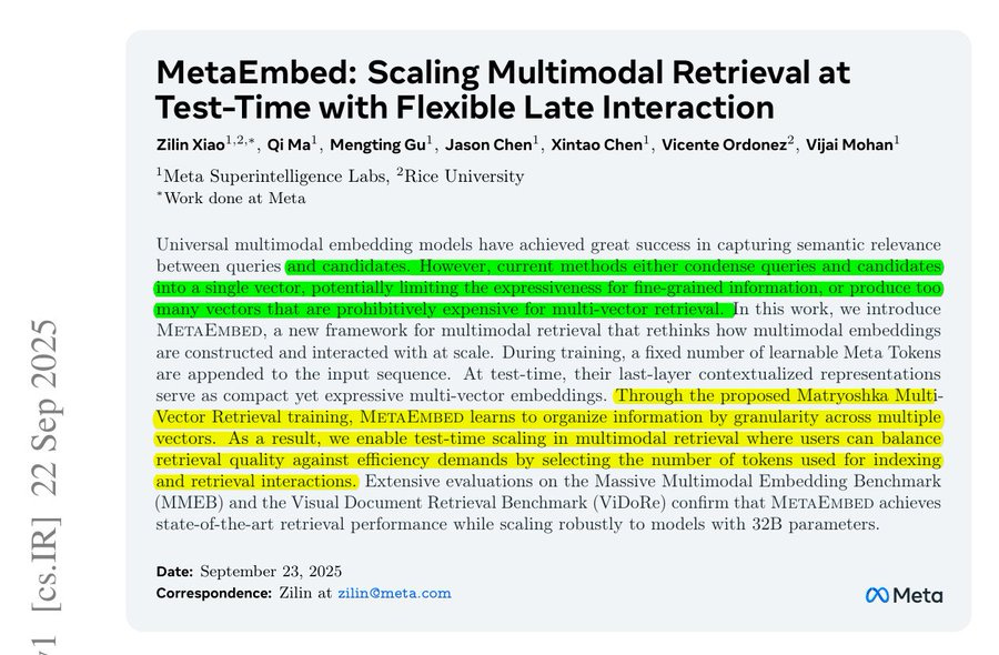
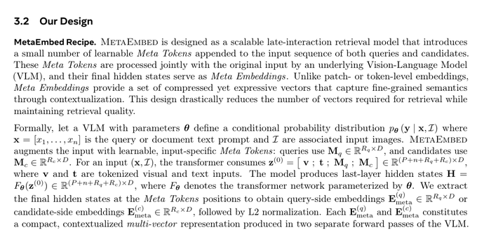
🗞️ MetaEmbed: Scaling Multimodal Retrieval at Test-Time with Flexible Late Interaction
Until now, people had two extremes. Either squeeze everything into 1 vector (fast but loses detail), or keep thousands of vectors (precise but insanely expensive). This paper shows a third path.
With just a handful of special “Meta Tokens”, you get nearly the same accuracy as the expensive setup but at a fraction of the cost. So you get the fine-grained accuracy of multi-vector retrieval without the huge cost, by compressing inputs into a tiny set of Meta Tokens.
The key win is that you can flexibly adjust accuracy vs. speed at test-time, no retraining needed.
So now you can literally dial in how much compute you want at test-time. e.g. use 1 token for blazing fast retrieval, or 64 tokens for maximum accuracy. And you don’t need to retrain anything.
This is such a great achievement, as most systems force you to lock in speed vs. accuracy during training. So when working with multimodal retrieval — searching across text, images, or both — this approach finally makes multi-vector practical at scale.
It gives you the accuracy benefits without blowing up memory or compute, and it gives you control to adjust budgets in production with zero retraining. It keeps multi-vector expressiveness but avoids storing every patch or word, because late interaction runs only over those Meta Tokens.
It stays practical at scale while keeping dual-encoder independence and controllable cost. With 16 query tokens and 64 candidate tokens, the 32B model reaches 78.7 Precision@1 on MMEB, while the 7B model hits 76.6.
The figure compares three different ways of doing multimodal retrieval and then shows how MetaEmbed changes the game. In the top left, you see the single-vector approach. Here the whole input, whether it’s text or image, is compressed into just one vector. That single vector is then matched against another single vector from a candidate. This keeps things cheap, but a lot of fine detail is lost because everything is squeezed down to one point.
In the top right, you see the traditional multi-vector approach. Instead of just one vector, every token from text or patch from an image gets its own vector. The model then matches them pairwise with max similarity scoring. This keeps detail, but the cost explodes, because thousands of comparisons have to be made.
In the bottom half, you see MetaEmbed’s idea. It introduces a small set of special Meta Tokens on both query and candidate sides.
These tokens summarize the input, but in a way that can be scaled step by step. They are organized in a nested, matryoshka-like structure, so the first tokens give a rough summary and extra tokens refine it.
During training, the system ensures each level is useful, so at test time you can flexibly choose how many tokens to use depending on whether you want speed or accuracy. So you see the trade-off. Single-vector is too coarse, multi-vector is too expensive, and MetaEmbed strikes a middle path with compact but flexible multi-vectors that scale smoothly with budget.
🚧 Why single or many vectors both hurt
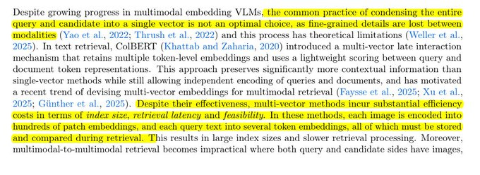
Single-vector systems crush everything into 1 number, so fine details vanish when text and image instructions get mixed in complex prompts and dense visuals. Classic multi-vector fixes fidelity but explodes cost, since thousands of query tokens must compare with thousands of candidate tokens, which makes multimodal-to-multimodal retrieval impractical for both training and inference.
⚙️ The Core Concepts
MetaEmbed appends a small, learnable set of Meta Tokens to the input, then uses their last-layer states as a compact multi-vector embedding that still captures fine detail through full-context processing. The same idea lives on both query and candidate sides, so encoders stay independent and the system keeps the retrieval-friendly dual-encoder workflow with only a handful of rich vectors per item.
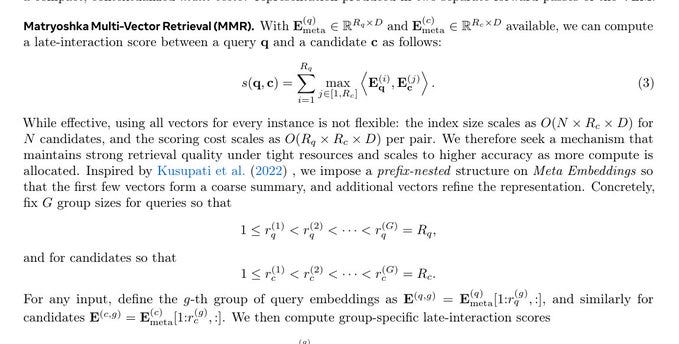
🪆 Matryoshka groups for test-time control
Training enforces a prefix-nested order over the Meta Embeddings, where the first few summarize coarsely and each extra token refines meaning, so any prefix length is a valid representation at test time. A system can pick (rq, rc) like (1,1), (2,4), (4,8), (8,16), or (16,64) on the fly, trading memory and latency for accuracy without retraining.
🧪 Training objective that keeps every prefix useful
Each group size gets its own contrastive objective in the same batch, which pushes even the smallest prefix to be discriminative while staying consistent as larger prefixes are added. The loss is a temperature-scaled InfoNCE over in-batch candidates plus a hard negative, summed across groups with simple weights, so optimization remains stable and fast.
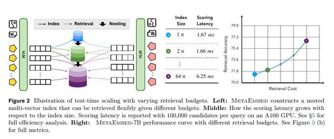
This figure shows why MetaEmbed is practical in real systems. On the left, it shows how Meta Tokens are stored in the index. Each candidate has a nested set of vectors, so you can flexibly choose how many to use when retrieving. This means you don’t have to re-train or rebuild the index to change cost.
In the middle, the table shows how latency grows with retrieval budgets. Even with 100,000 candidates per query, using only 1 token gives a latency of 1.67 ms, and even the largest budget with 64 tokens only takes 6.25 ms. That’s a very small increase considering how much accuracy improves.
On the right, the curve shows this trade-off directly. As you increase retrieval cost, retrieval accuracy climbs steadily. The important part is that the gains are smooth and controllable, so you can set a budget depending on whether you want more speed or more accuracy.
Main takeaway; MetaEmbed gives you a scalable knob:
tiny cost when you need speed, and much higher accuracy when you can afford a slightly larger budget, without retraining or rebuilding the system.
🎛️ The budget knob, accuracy versus cost
Indexing can store only the first rc candidate tokens to save memory, and queries can use only the first rq tokens to hit a latency target, then scoring compares those prefixes with a late-interaction max-sim and sums over query tokens. Small budgets give fast first-stage retrieval, larger budgets give higher precision, and switching budgets needs no retraining because the nested structure was learned during training.
🗞️ Video models are zero-shot learners and reasoners
Brilliant GoogleDeepMind paper shows that a single video model can handle many vision tasks from simple prompts, with no extra training. The authors test Veo 3 on 62 tasks across 18,384 videos, and it works on a wide mix of jobs.
Shows broad 0-shot perception, editing, and simple visual reasoning without task specific training. The big deal is that 1 general model can do many different vision tasks just by changing the prompt.
All these means, we need fewer special purpose models and simpler workflows across vision problems. Older vision setups need a separate model per job, here they give 1 input image plus a short instruction to a video generator.
0-shot means no fine tuning, the model reads the instruction and outputs frames that show the answer. It handles perception tasks like edge finding, segmentation which means coloring each object separately, super resolution, deblurring, denoising, and low light fixes.
It also shows basic physics sense like buoyancy, air resistance, and optics, and it keeps track of the scene even when the camera moves. It edits images and scenes, removing backgrounds, changing style or pose, composing scenes, and simulating tool use.
Its frame by frame process supports reasoning, like planning routes, completing symmetry patterns, and solving simple mazes. On measured tests it comes close to strong image editors for segmentation and edge detection, and it beats its prior version on maze solving. Weak spots remain for depth maps and surface normals which are surface direction labels, plus following force arrows and some physics, so results can be uneven across tasks.
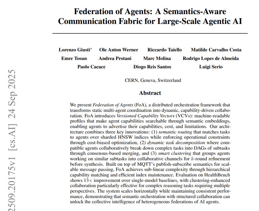
🗞️ Federation of Agents: A Semantics-Aware Communication Fabric for Large-Scale Agentic AI
The paper builds a simple system that finds and coordinates the right AI agents for each job. It reports 13x better results on a hard healthcare test than the best single model.
It shows that searchable skill profiles and capability-aware routing beat a one-model setup by a wide margin. It turns messy “who should do what” decisions into a clear procedure that respects rules and budgets.
It proves the point with a tough benchmark and a practical stack that can scale across many agents. Each agent has a small profile called a Versioned Capability Vector that lists skills, limits, cost, and rules.
These profiles are turned into numbers so the system can search them fast. When a big task comes in, an orchestrator splits it into clear subtasks and picks agents for each part.
The pick uses meaning match, policy checks, and budget fit to choose the best team. Agents put work in a shared channel, review each other, vote, and improve the draft over a few rounds.
The orchestrator then joins the subtask answers using the plan of what depends on what. Messages move using Message Queuing Telemetry Transport publish or subscribe, which handles many agents and flaky links well. The result is faster help, safer choices, and steady costs when many different agents work together.
That’s a wrap for today, see you all tomorrow.


