What factors influence chunk size

Browse all previously published AI Tutorials here.

Table of Contents

• What factors influence chunk size

• Chunk Size Considerations in Transformer-Based LLMs

  • Tokenization and Chunk Size

  • Training Data Batching and Sequence Length

  • Inference Windowing and Decoding Chunk Size

Chunk Size Considerations in Transformer-Based LLMs

Overview: “Chunk size” can refer to how text is segmented at various stages of an LLM pipeline – from tokenization granularity, to training batch sequence lengths, to inference windowing during generation. Each stage involves trade-offs in memory use, latency, and GPU utilization. Below, we examine how chunk size choices affect vocabulary efficiency and model performance (tokenization), training throughput and convergence (batching), and inference speed (windowing), drawing on 2024–2025 insights.

Tokenization and Chunk Size

Tokenization determines how text is broken into tokens (subword units, bytes, characters, etc.), influencing the total token count (chunk length) for a given input and the vocabulary size. Key trade-offs include:

• Vocabulary Size vs. Sequence Length: Using larger tokens (e.g. whole words or long subwords) reduces the number of tokens per input (shorter sequences), but requires a larger vocabulary. A larger vocab means more embedding parameters and potential memory overhead, whereas smaller tokens (characters or small subwords) inflate sequence length and computation. For example, a multilingual study found that using an English-centric subword tokenizer for other languages made tokenized sequences up to 15× longer than necessary, greatly increasing inference cost and latency (HERE). It also required about 3× larger vocabulary to avoid severe performance drops – inefficient tokenization can raise training costs by 68% due to longer sequences .

• Compression vs. Model Performance: Intuitively, one might expect that chunking text into as few tokens as possible (high compression) is optimal. However, recent research shows this isn’t strictly true. A 2024 paper introduced PathPiece, an extreme tokenizer that minimizes token count for a given vocab size, and tested the hypothesis “fewer tokens = better performance.” In practice, condensing text into minimal tokens did not always yield better downstream accuracy (Tokenization Is More Than Compression). This finding “casts doubt” on the idea that tokenization quality is solely about compression . In fact, moderate subword segmentation often works best – too coarse and the model loses granularity, too fine and the sequence is overly long.

• Downstream Impact: The choice of tokenizer can significantly affect an LLM’s final accuracy and efficiency. One comprehensive 2024 study trained 24 LLMs (2.6B params) with different tokenizers and showed that tokenizer differences lead to noticeable changes in model performance and training cost (HERE) . Notably, common intrinsic metrics like token fertility (tokens per word) didn’t always predict downstream performance . This means engineers must empirically test tokenizers: a tokenizer that yields shorter texts isn’t guaranteed to produce a better model if it, for instance, splits words in unnatural ways for the model’s learning.

• Memory and Efficiency: Finer tokenization (small chunks) means a smaller embedding matrix (fewer unique tokens) but longer sequences to process. Coarser tokenization (large chunks) yields shorter sequences but a huge embedding/vocabulary matrix. Large vocabularies can be very memory-hungry – e.g. a multilingual model might need hundreds of thousands of tokens, leading to billions of parameters just in embeddings and output layers (HERE). Researchers have found that many subword vocabularies are inefficiently used – up to 34% of BPE tokens can be near-duplicates, wasting space . This motivates alternative tokenization methods that maintain efficiency with fewer unique tokens.

• Subword vs. Byte-Pair vs. Alternatives: Subword tokenization (including BPE) is the de-facto standard for LLMs, balancing vocabulary size and sequence length. BPE, originally a data compression method, merges frequent character sequences to reduce token count. However, as noted, maximal compression via BPE isn’t always best for the model (Tokenization Is More Than Compression). Alternatives include unigram language model tokenizers (e.g. SentencePiece), character-level models, or even byte-level tokenization. Byte-level (or character) approaches eliminate out-of-vocabulary issues and simplify tokenization across languages, but dramatically increase sequence lengths, which can hurt speed due to the transformer’s quadratic attention cost. Recent papers explore tokenizer-free architectures: for example, T-FREE (2024) encodes words as combinations of character trigram patterns, reducing embedding layer size by >85% while staying competitive in downstream tasks . By using sparse multi-character representations, it addresses tokenizer drawbacks like large embedding tables and poor cross-lingual transfer . Another line of work compresses text with neural encoders – one 2024 study trained LLMs on neurally compressed text, achieving much shorter sequences than subwords. The compressed tokens yielded faster inference (fewer autoregressive steps) at the cost of slightly higher perplexity for a given model size (Training LLMs over Neurally Compressed Text | OpenReview). Such methods highlight the engineering trade-off: aggressively shorter token sequences can boost speed (and reduce memory per sequence) but may require a larger model or more training to reach the same accuracy .

In summary, tokenization chunk size is a balance between compression and information loss. Engineering choices here affect how efficiently the model represents text: a well-chosen subword tokenizer can cut sequence length by ~40% without hurting performance (HERE), whereas a poorly suited tokenizer (e.g. wrong language or domain) can explode sequence lengths and degrade both speed and accuracy. Modern LLM pipelines therefore carefully evaluate tokenization on target data and sometimes opt for hybrid or learned tokenization strategies to maximize downstream performance per token.

Training Data Batching and Sequence Length

During training, chunk size usually refers to the sequence length of training examples (the number of tokens per sample or per batch segment) and how data is batched. This affects memory usage, training speed (steps/second), and how quickly the model converges. Important considerations:

• Batch Size and Gradient Accumulation: Large batch sizes are desirable for faster training and stable convergence in LLMs (following scaling laws). Recent work notes that state-of-the-art LLM training often uses the equivalent of tens of millions of tokens per batch to fully utilize clusters of GPUs . However, a single GPU cannot hold such a batch if sequences or models are large. Gradient accumulation is a common workaround: the batch is split into many micro-batches that are run sequentially on hardware, accumulating gradients before an update . This allows an effective large batch without requiring huge memory at once. The trade-off is increased iteration time (less parallelism) and potential communication overhead when summing gradients. Empirically, large effective batch sizes (with accumulation) can improve training efficiency and even convergence quality for LLMs , but going too large can also introduce optimization difficulties (plateauing or generalization issues) if not tuned. Engineers must balance batch size for throughput against the point of diminishing returns for model quality.

• Throughput and GPU Utilization: Packing more tokens per batch (either via longer sequences or more sequences) improves GPU utilization – up to the limit of GPU memory and bandwidth. There’s often a U-shaped curve for tokens/sec vs. batch size: initially throughput increases with batch size, but beyond a certain size, it plateaus or even dips if it triggers out-of-memory or increased overhead. Notably, sequence packing strategies can significantly boost effective batch size. Instead of padding all sequences to a fixed length, packing concatenates multiple shorter examples into one long sequence (with proper masking) so that less space is wasted on padding (Enhancing Training Efficiency Using Packing with Flash Attention) . This increases the useful tokens per batch and keeps GPUs busy with real data. Dynamic padding (bucketing sequences by similar lengths) and packing are widely used to maximize training tokens processed per step.

( Enhancing Training Efficiency Using Packing with Flash Attention) In fact, a 2024 study demonstrated that minibatch packing almost doubles training throughput (in tokens/sec) compared to naive padding, and significantly lowers peak memory usage per GPU. In the figure below, the red curve (packed sequences) sustains much higher throughput as batch size grows, whereas the blue curve (padding each sequence) hits memory limits (OOM) at smaller batch sizes. This illustrates that by concatenating smaller chunks into a larger one, training can scale to bigger batches without running out of memory, achieving better hardware utilization.

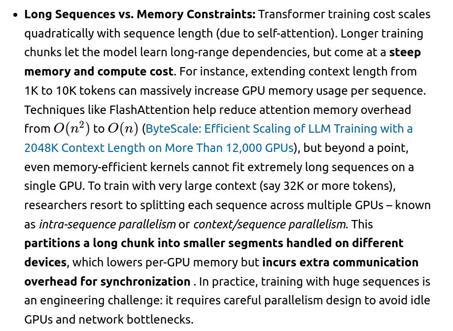
• Communication Overhead: In distributed training, chunk size can also impact communication. If using data parallelism (each GPU gets different samples), larger batches mean more gradients to all-reduce between GPUs – usually a minor cost relative to computation, unless batch size is extremely large or network is slow. On the other hand, if using model or pipeline parallelism, the chunk (sequence) may be split across GPUs (as mentioned for long contexts) or layers spread across GPUs. In those cases, synchronization at every layer or segment can become a bottleneck (Glinthawk: A Two-Tiered Architecture for High-Throughput LLM Inference). For example, with tensor (model) parallelism, after each layer’s partial computations, GPUs must exchange results (AllGather) – if the sequence chunk is long, this happens many times per sample, and small per-step compute can make communication the dominant cost . One mitigation is asynchronous or overlapped execution (pipelining micro-batches through model shards) to hide latency . Overall, the larger the chunk of work each GPU must synchronize (either a huge batch in data-parallel or a long sequence in pipeline-parallel), the more one must design around communication delays. Recent systems like ByteScale (2025) introduce optimized parallelism to handle variable sequence lengths without idling GPUs, combining data- and context-parallel approaches efficiently (ByteScale: Efficient Scaling of LLM Training with a 2048K Context Length on More Than 12,000 GPUs) . The goal is to keep all GPUs busy even when chunk sizes differ (since real datasets have a skewed length distribution), to maximize throughput.

• Convergence and Long-Range Learning: Using longer training chunks can help models learn dependencies across a broader context (beneficial for long text understanding). Some curricula increase sequence length as training progresses. However, longer sequences per batch can also mean fewer optimization steps for a fixed corpus size (since each step consumes more tokens), potentially slowing initial convergence. Researchers must monitor if larger chunk sizes are actually improving validation metrics or if the model could get similar results with shorter chunks (and more frequent updates). In practice, a mix of chunk sizes might be used (e.g. shorter sequences for early training, longer for fine-tuning on long-context tasks). The Chinchilla scaling laws imply that for a given model size and token budget, there is an optimal batch size and maybe an optimal sequence length – overshooting it wastes computation. Recent experiments at very long contexts (50k+ tokens) show that beyond a certain length, returns diminish unless the model and data genuinely require that context. Thus, engineers weigh faster iteration (with shorter sequences) against more comprehensive context per sample (with longer sequences) to find a sweet spot for training efficiency.

Inference Windowing and Decoding Chunk Size

During inference (generation), chunk size relates to how much context is processed in one go – for example, the model’s attention window and how we batch tokens for autoregressive decoding. The practical goals are to maximize throughput (tokens generated per second) while respecting latency constraints and GPU memory limits. Here’s how chunking comes into play:

• Autoregressive Decoding Cost: In generation, transformers produce one token at a time, and each new token attends to the entire prior context (all previous tokens in the sequence). This means as the output grows, each step becomes progressively more expensive: if a model has generated k tokens so far, the next token involves an attention computation over k keys/values. A longer context (chunk) thus increases per-token latency. Caching helps – the model doesn’t recompute earlier layers for past tokens, but the attention still must read all k cached keys/values. When k is large, attention over a long key-value cache can become memory-bandwidth bound, i.e. just reading all those past tokens’ embeddings each step hurts latency (Efficient Generative LLM Inference with Recallable Key-Value Eviction). In other words, long contexts slow down throughput because of the O(n) attention work per token. Recent NeurIPS 2024 work on key-value eviction noted that beyond a certain length, the model spends a lot of time on memory accesses for the cache, so selectively trimming or compressing the cache (chunking the context) can improve speed . This is an active area: strategies like sliding windows, recurrent memory, or chunked attention aim to bound the “effective” context size to a fixed window (e.g. last 2048 tokens) so that each new token’s computation is limited. The trade-off is that if you discard or summarize older tokens, the model may lose some context – so systems decide how much context can be dropped without impacting output quality for the task at hand.

• Context Length Constraints: Every model has a maximum context length (e.g. 4K tokens, 32K tokens, etc.), which is essentially a hard chunk size limit for inference. If the input prompt or generated text exceeds this, one must use windowing techniques to handle it. Practical solutions include chunking the input into smaller segments and processing sequentially (for tasks like summarization of a long document, feed the text in pieces), or using models specifically fine-tuned to longer contexts. If using fixed-window models on longer text, developers might generate or process in chunks: for example, summarize each chunk then summarize the summaries, or use retrieval (fetch relevant pieces into context as needed). These approaches trade fidelity for feasibility. Another approach is overlapping windows: e.g. read 1024 tokens, then slide 512 tokens and read the next 1024, so that some context carries over. This can help preserve continuity but increases computation (some overlap is processed twice). In all cases, there is a latency hit for very long inputs, since the model must be run multiple times on chunks. Research from late 2024 on ultra-long context models shows that training with efficient attention or recurrence can extend context lengths (128K, 1M tokens) (ByteScale: Efficient Scaling of LLM Training with a 2048K Context Length on More Than 12,000 GPUs) , but serving these models requires enormous memory and careful batching (sometimes splitting the context across many GPUs). Thus, production systems often prefer to stay within the model’s native window when possible or use hybrid strategies (like summarizing long context into a shorter prompt).

• Batching and Latency Trade-offs: In multi-user inference (serving many queries), chunking also refers to batching multiple requests together. Batching improves GPU utilization and throughput – the model can score or generate several tokens in parallel – but it increases individual request latency because each query may wait for others in the batch (Glinthawk: A Two-Tiered Architecture for High-Throughput LLM Inference). A recent study succinctly notes: “Batching prompts improves throughput, but exacerbates latency. In general, inference throughput and latency are conflicting goals.” . This trade-off is crucial in real-world LLM services. Large batch decoding (processing many tokens across different sequences at once) achieves a high tokens/sec rate, maximizing GPU usage, but if a request is alone or needs very fast response, forcing it to wait for a batch would hurt its latency. Engineers address this by dynamic batching – grouping requests on the fly if they arrive around the same time, and tuning batch sizes to balance utilization vs. delay. For instance, an online system might batch all tokens that are ready to generate at a given moment (every 10 ms, say) to keep the GPU busy, but will immediately process a request if it’s been waiting too long. This dynamic windowing ensures no request gets stuck indefinitely waiting to fill a large batch. There’s also a notion of optimal batch size per hardware – beyond a certain batch size, the GPU may saturate and not yield extra throughput, so batching more only adds latency with no throughput gain.

• Hybrid Prefill/Decode Scheduling: Modern LLM inference frameworks use two-phase processing for generation: a prefill phase (process the prompt in full) and a decode phase (generate tokens one by one). These phases have different compute characteristics – prefill is heavy matrix multiplication over a long input (compute-bound), decode is repetitive light compute with lots of memory access to the cache (memory-bound) (POD-Attention: Unlocking Full Prefill-Decode Overlap for Faster LLM Inference) . To optimize throughput, systems intermix work from different requests. For example, while one long prompt is being processed, another request’s decode steps might run in parallel on other hardware resources. Advanced schedulers implement hybrid batching, combining prompt tokens from some requests and generated tokens from others in a single batch operation . This ensures the GPU is doing a mix of compute- and memory-intensive work simultaneously, thus using both ALUs and memory bandwidth efficiently . A key technique here is chunked prefill: if one request has an extremely long prompt, the scheduler can split the prompt into smaller chunks (e.g. process 500 tokens of it at a time) and between those chunks, do decoding for other requests . By windowing the prompt ingestion like this, the system avoids delaying all other queries until that one large prompt finishes. Essentially, no single inference chunk should monopolize the GPU for too long – breaking up long contexts and interweaving generation steps from multiple requests improves overall throughput and lowers tail latency . BatchLLM (2024) and similar systems explicitly group requests with common prefixes and different lengths to maximize such overlap, reusing cached key-values for shared prefixes and scheduling shorter decoding-heavy requests first so longer prompts can be pipelined in chunks (BatchLLM: Optimizing Large Batched LLM Inference with Global Prefix Sharing and Throughput-oriented Token Batching) . These optimizations significantly increase GPU utilization for batched inference, often outperforming naive FIFO scheduling by eliminating idle or “valley” periods where the GPU waits for a long sequence .

• Memory vs. Speed in Decoding: Another factor is the GPU memory allocated for key/value caches during generation. A model with maximum context N will allocate memory for N keys and values per layer. If we don’t actually need N tokens of context for a given query, that memory is reserved but unused. Some inference servers dynamically adjust the effective context length per batch. For instance, if the longest prompt in a batch is 500 tokens and we will generate at most 500 more, they might limit the attention mask to 1000 and not use the full 8K capacity, to save memory and allow larger batch sizes. On the flip side, if you have many long-running generations, the memory for their caches accumulates, possibly limiting how many can batch together. There’s a trade-off: keeping longer context available avoids cache misses (needing to recompute from scratch if a token falls out of the window), but consumes memory. Solutions like evicting old cache entries can free memory (so more or bigger batches fit) at the cost of recomputing those when needed (Efficient Generative LLM Inference with Recallable Key-Value Eviction). The optimal chunking may depend on the application’s tolerance for recomputation vs. latency. For example, a chatbot might safely discard oldest context beyond a few thousand tokens to serve more users simultaneously, whereas a code completion tool might keep the full context of a file in cache for accuracy, accepting a slower single-user throughput.

In summary, inference chunking is about managing context and batches to maximize throughput without violating real-time constraints. High-throughput settings (bulk processing of many documents) will use large chunks and batches to fully utilize GPUs (BatchLLM: Optimizing Large Batched LLM Inference with Global Prefix Sharing and Throughput-oriented Token Batching) , whereas interactive settings window the process to keep latency low for each user. Techniques like hybrid batching, sliding windows, and cache management all stem from the core trade-offs introduced by chunk size: a larger chunk (more tokens at once) improves efficiency up to a point, but too large can bottleneck either compute (if sequential) or memory. Optimizing LLM inference has therefore become an art of chunk scheduling, ensuring that at each step the model is working on an appropriately sized window of data for the hardware to stay busy but responsive.

References: The insights above are drawn from recent (2024–2025) research and engineering reports on LLM efficiency, including studies on tokenizer impact (HERE), training optimization methods (ByteScale: Efficient Scaling of LLM Training with a 2048K Context Length on More Than 12,000 GPUs), and high-throughput inference system designs (Glinthawk: A Two-Tiered Architecture for High-Throughput LLM Inference). These works emphasize that there is no one-size-fits-all chunk size – it’s a knob to tune for each stage. By understanding the trade-offs (compression vs. model capacity, batch size vs. memory, and throughput vs. latency), practitioners can make informed decisions to maximize their Transformer-based LLM’s performance within resource constraints.