
Why Bootstrapping is useful and Implementation of Bootstrap Sampling in Random Forests


Link to full Code in Kaggle and Github
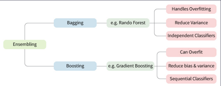
First a note on Ensemble Learning
The general principle of ensemble methods is to construct a linear combination of some model fitting method, instead of using a single fit of the method. The main principle behind the ensemble model is that a group of weak learners come together to form a strong learner, thus increasing the accuracy of the model.When we try to predict the target variable using any machine learning technique, the main causes of difference in actual and predicted values are noise, variance, and bias. Ensemble helps to reduce these factors (except noise, which is irreducible error). The noise-related error is mainly due to noise in the training data and can’t be removed. However, the errors due to bias and variance can be reduced. The total error can be expressed as follows:
Total Error = Bias + Variance + Irreducible Error
Why we do Bootstrap re-sampling
Bootstrapping resamples the original dataset with replacement many thousands of times to create simulated datasets. This process involves drawing random samples from the original dataset. Through bootstrapping you are simply taking samples over and over again from the same group of data (your sample data) to estimate how accurate your estimates about the entire population (what really is out there in the real world) is.
If you were to take one sample and make estimates on the real population, you might not be able to estimate how accurate your estimates are — we only have one estimate and have not identified how this estimate varies with different samples that we might have encountered.
Bootstrap Aggregation (or Bagging for short), is a simple and very powerful ensemble method.
An ensemble method is a technique that combines the predictions from multiple machine learning algorithms together to make more accurate predictions than any individual model.
Bootstrap Aggregation is a general procedure that can be used to reduce the variance for those algorithm that have high variance. An algorithm that has high variance are decision trees, like classification and regression trees (CART).
Decision trees are sensitive to the specific data on which they are trained. If the training data is changed (e.g. a tree is trained on a subset of the training data) the resulting decision tree can be quite different and in turn the predictions can be quite different.
Bagging is the application of the Bootstrap procedure to a high-variance machine learning algorithm, typically decision trees.
Another major drawback associated with the tree classifiers is that they are unstable. That is, a small change in the training data set can result in a very different tree. The reason for this lies in the hierarchical nature of the tree classifiers. An error that occurs in a node at a high level of the tree propagates all the way down to the leaves below it.
And so Bagging (bootstrap aggregating) can reduce the variance and improve the generalization error performance. The basic idea is to create B variants, X1, X2 , . . . , XB , of the training set X, using bootstrap techniques, by uniformly sampling from X with replacement. For each of the training set variants Xi , a tree Ti is constructed. The final decision for the classification of a given point is in favor of the class predicted by the majority of the subclassifiers Ti , i = 1, 2, . . . , B.
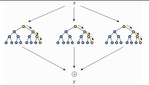
Finally Principle of Random Forest with Bootstrapping
The below text is taken from this source
Firstly, using Bootstrap resampling technique, multiple samples are randomly selected from the original training sample set x to generate a new training sample set. Then, multiple decision trees are constructed to form random forest. Finally, the random forest averages the output of each decision tree to determine the final filling result y. Due to the Bootstrap used in the random decision tree generation process, all samples are not used in a decision tree and the unused samples are called out of band (OOB). Through out of band, the accuracy of the tree can be evaluated. The other trees are evaluated according to the principle and finally average the results.
Now our Code Implementations
There will be some functions that start with the word “grader” ex: grader_sampples(), grader_30().. etc, we should not change those function definition. Every Grader function has to return True.
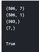
x.shape  (506, 13)
y.shape  (506,)
Task 1
Creating samples — Randomly create 30 samples from the whole boston data points
Creating each sample: Consider any random 303(60% of 506) data points from whole data set and then replicate any 203 points from the sampled points
For better understanding of this procedure lets check this examples, assume we have 10 data points [1,2,3,4,5,6,7,8,9,10], first we take 6 data points randomly , consider we have selected [4, 5, 7, 8, 9, 3] now we will replicate 4 points from [4, 5, 7, 8, 9, 3], consder they are [5, 8, 3,7] so our final sample will be [4, 5, 7, 8, 9, 3, 5, 8, 3,7]
Create 30 samples
Note that as a part of the Bagging when we are taking the random samples make sure each of the sample will have different set of columns Ex: Assume we have 10 columns[1 ,2 ,3 ,4 ,5 ,6 ,7 ,8 ,9 ,10] for the first sample we will select [3, 4, 5, 9, 1, 2] and for the second sample [7, 9, 1, 4, 5, 6, 2] and so on… Make sure each sample will have atleast 3 feautres/columns/attributes
Step — 1 — Creating samples
Creating 30 samples

Step — 2 of Task-1
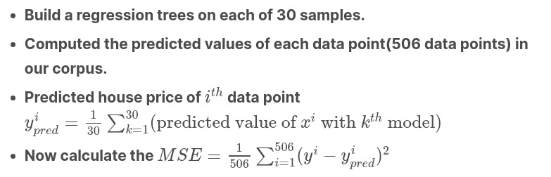
Building High Variance Models on each of the sample and finding train MSE value
Flowchart for Building regression trees
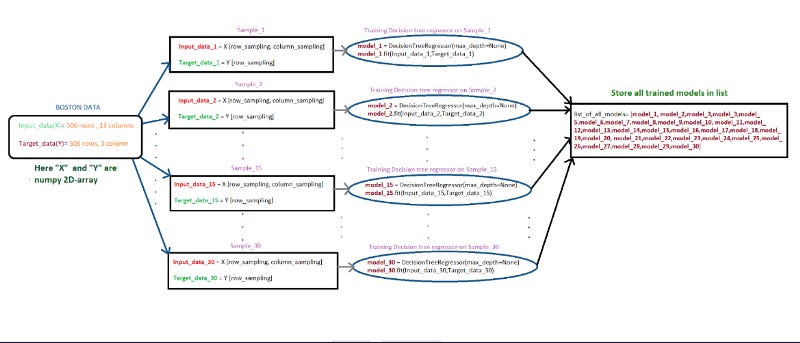
list_of_all_models_decision_tree = []
for i in range(0, 30):
model_i = DecisionTreeRegressor(max_depth=None)

model_i.fit(list_input_data[i], list_output_data[i])

list_of_all_models_decision_tree.append(model_i)
Flowchart for calculating MSE
After getting predicted_y for each data point, we can use sklearns mean_squared_error to calculate the MSE between predicted_y and actual_y.
Calculating MSE
Step — 3 of Task-1
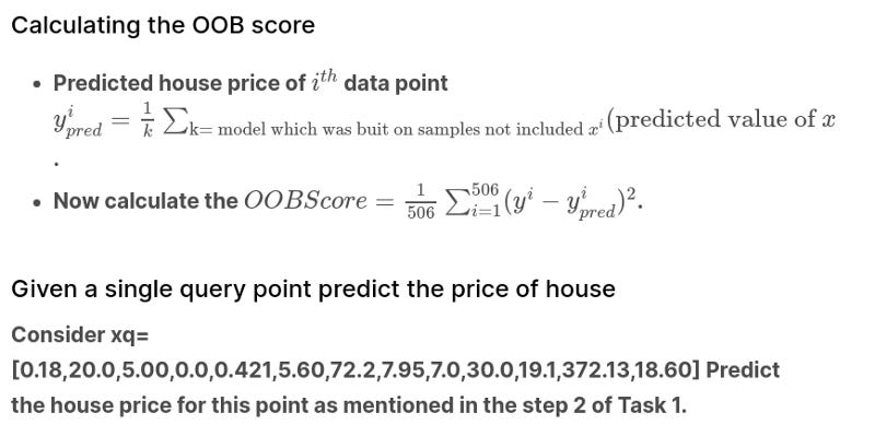
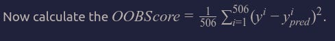
Flowchart for calculating OOB score
Further notes on above OOB calculation
The key point is that the OOB sample rows were passed through every Decition Treee that did not contain those specific OOB sample rows during the bootstrapping of training data.
OOB error is simply the error on samples that were not seen during training.
OOB Scoring is very useful when I dont have a large dataset and thereby if I split that dataset into training and validation set — will result in loss of useful data that otherwise could have been used for training the models. Hence in this case, we decide to extract some of the training data as the validation set by using only those data-points that were not used for training a particular sample-set.
Task 2
Computing CI of OOB Score and Train MSE
Repeat Task 1 for 35 times, and for each iteration store the Train MSE and OOB score
After this we will have 35 Train MSE values and 35 OOB scores
using these 35 values (assume like a sample) find the confidence intravels of MSE and OOB Score
we need to report CI of MSE and CI of OOB Score
Note: Refer the Central_Limit_theorem.ipynb to check how to find the confidence intravel
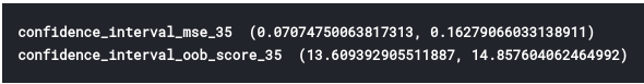
Observation / Interpretation of above Confidence Interval
By definition we know the interpretation of a 95% confidence interval for the population mean as — If repeated random samples were taken and the 95% confidence interval was computed for each sample, 95% of the intervals would contain the population mean.
So in this case
MSE — There is a 95% chance that the confidence interval of (0.05732086175441538, 0.11667646077442519) contains the true population mean of MSE.
OOB Score — There is a 95% chance that the confidence interval of (13.274222499705303, 14.427942855729313) contains the true population mean of OOB Score.
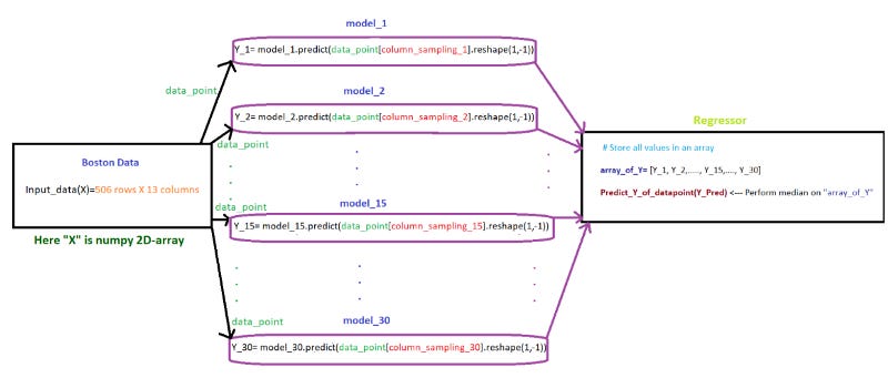
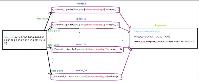
Task 3 (send query point “xq” to 30 models)
We created 30 models by using 30 samples in TASK-1. Here, we need send query point “xq” to 30 models and perform the regression on the output generated by 30 models
Flowchart for Task 3
18.7
Link to full Code in Kaggle and Github
References:
Brownlee, Jason. “A Gentle Introduction to the Bootstrap Method”. Machine Learning Mastery, May 25th, 2018. https://machinelearningmastery.com/a-gentle-introduction-to-the-bootstrap-method/. Date accessed: May 24th, 2020.
Kulesa, Anthony et al. “Sampling distributions and the bootstrap.” Nature methods vol. 12,6 (2015): 477–8. doi:10.1038/nmeth.3414
http://faculty.washington.edu/yenchic/17Sp_403/Lec5-
bootstrap.pdfhttps://web.as.uky.edu/statistics/users/pbreheny/764-F11/notes/12-6.pdf
http://www.stat.rutgers.edu/home/mxie/rcpapers/bootstrap.pdf