Why we do log transformation of variables and interpretation of Logloss

What is Log Transformation

Original number = x

Log Transformed number x=log(x)

For zeros or negative numbers, we can’t take the log; so we add a constant to each number to make them positive and non-zero.

Each variable x is replaced with log(x), where the base of the log is left up to the analyst. It is considered common to use base 10, base 2 and the natural log ln.

The log transformation, a widely used method to address skewed data, is one of the most popular transformations used in Machine Learning.

One of the main reasons for using a log scale is that log scales allow a large range to be displayed without small values being compressed down into the bottom of the graph.

This process is useful for compressing the y-axis when plotting histograms. For example, if we have a very large range of data, then smaller values can get overwhelmed by the larger values. Taking the log of each variable enables the visualization to be clearer.

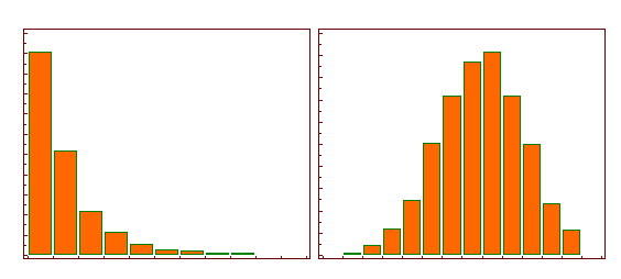
The following illustration shows the histogram of a log-normal distribution (left side) and the histogram after logarithmic transformation (right side), transforming a highly skewed variable into one that is more approximately normal.

Why do we do log transformations of variables?

Reason-1 (when working with skewed datasets)

Skewness is a measure of the symmetry in a distribution. A symmetrical data set will have a skewness equal to 0. So, a normal distribution will have a skewness of 0. Skewness essentially measures the relative size of the two tails.

When our original continuous data do not follow the bell curve, we can log transform this data to make it as “normal” as possible so that the statistical analysis results from this data become more valid. In other words, the log transformation reduces or removes the skewness of our original data. The important caveat here is that the original data has to follow or approximately follow a log-normal distribution. Otherwise, the log transformation won’t work.

When the variables span several orders of magnitude. Income is a typical example: its distribution is “power law”, meaning that the vast majority of incomes are small and very few are big. This type of “fat tailed” distribution is studied in a logarithmic scale because of the mathematical properties of the logarithm:

Logarithm naturally reduces the dynamic range of a variable so the differences are preserved while the scale is not that dramatically skewed. Imagine some people got 100,000,000 loans and some got 10000 and some 0. Any feature scaling will probably put 0 and 10000 so close to each other as the biggest number anyway pushes the boundary. Logarithm solves the issue.

If you take values 1000,000,000 and 10000 and 0 into account. In many cases, the first one is too big to let others be seen properly by your model. But if you take logarithm you will have 9, 4 and 0 respectively. As you see the dynamic range is reduced while the differences are almost preserved. It comes from any exponential nature in your feature.

Reason-2 ( capture non-linear relationships, while preserving the linear model)

Logarithmically transforming variables in a regression model is a very common way to handle situations where a non-linear relationship exists between the independent and dependent variables.3 Using the logarithm of one or more variables instead of the un-logged form makes the effective relationship non-linear, while still preserving the linear model.

Reason-3 (when underlying data itself is lognormal)

People may use logs because they think it compresses the scale or something, but the principled use of logs is that you are working with data that has a lognormal distribution. This will tend to be things like salaries, housing prices, etc, where all values are positive and most are relatively modest, but some are very large.

If you can take the log of the data and it becomes normalish, then you can take advantage of many features of a normal distribution, like well-defined mean, standard deviation (and hence z-scores), symmetry, etc.

Similarly, addition of logs is the same as multiplication of the un-log’d values. Which means that you’ve turned a distribution where errors are additive into one where they’re multiplicative (i.e. percentage-based). Since techniques like OLS regression require a normal error distribution, working with logs extends their applicability from additive to multiplicative processes.

**Reason-4 (**ratio datasets)

Yet another reason why logarithmic transformations are useful comes into play for ratio data, due to the fact that log(A/B) = -log(B/A). If you plot a distribution of ratios on the raw scale, your points fall in the range (0, Inf). Any ratios less than 1 will be squished into a small area of the plot, and furthermore, the plot will look completely different if you flip the ratio to (B/A) instead of (A/B). If you do this on a logarithmic scale, the range is now (-Inf, +Inf), meaning ratios less than 1 and greater than 1 are more equally spread out. If you decide to flip the ratio, you simply flip the plot around 0, otherwise, it looks exactly the same. On a log scale, it doesn’t really matter if you show a ratio as 1/10 or 10/1, which is useful when there’s not an obvious choice about which it should be.

Drawbacks of Log Transformation

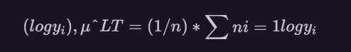
Once the data is log-transformed, many statistical methods, including linear regression, can be applied to model the resulting transformed data. For example, the mean of the log-transformed observations

​is often used to estimate the population mean of the original data by applying the anti-log (i.e., exponential) function to obtai

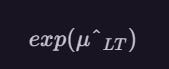
However, this inversion of the mean log value does not usually result in an appropriate estimate of the mean of the original data.

It is also more difficult to perform hypothesis testing on log-transformed data.

Interpretation of Log Loss

Log Loss is the most important classification metric based on probabilities.

It’s hard to interpret raw log-loss values, but log-loss is still a good metric for comparing models.

For any given problem, a lower log-loss value means better predictions.

The concept of Log Loss is a modified form of something called the Likelihood Function. In fact, Log Loss is

-1 * the log of the likelihood function.

So, lets understand the likelihood function.

The likelihood function answers the question “How likely did the model think the actually observed set of outcomes was.”

Example

A model predicts probabilities of [0.8, 0.4, 0.1] for three cases of medical patients of detecting cancer or Not. The first two cases were indeed found to be positive with cancer, and the last one was NOT. So the actual outcomes could be represented numerically as [1, 1, 0].

Let’s step through these predictions one at a time to iteratively calculate the likelihood function.

The first case was YES for Cancer, and the model said that was 80% likely. So, the likelihood function after looking at one prediction is 0.8.

The second case was also YES, and the model said that was 40% likely.

There the rule of probability of multiple independent events, both occurring is the product of their individual probabilities. So, we get the combined likelihood from the first two predictions by multiplying their associated probabilities. That is 0.8 * 0.4, which happens to be 0.32.

Now we get to our third prediction. This patient was Negative for Cancer. The model said it was 10% likely to being Positive for Cancer. That means it was 90% likely to not having Cancer. So, the observed outcome of not having cancer was 90% likely according to the model. So, we multiply the previous result of 0.32 by 0.9.

We could step through all of our predictions. Each time we’d find the probability associated with the outcome that actually occurred, and we’d multiply that by the previous result. That’s the likelihood.

From Likelihood to Log Loss

Each prediction is between 0 and 1. If you multiply enough numbers in this range, the result gets so small that computers can’t keep track of it. So, as a clever computational trick, we instead keep track of the log of the Likelihood. This is in a range that’s easy to keep track of. We multiply this by negative 1 to maintain a common convention that lower loss scores are better.

log loss penalizes quite high for an incorrect or a far-off prediction, i.e. log loss punishes you for being very sure and very wrong